¶ Profile Type Maps
To have the profile types calculated for the model, Build Profile Type Map must be selected in the Tools menu. A new window opens.
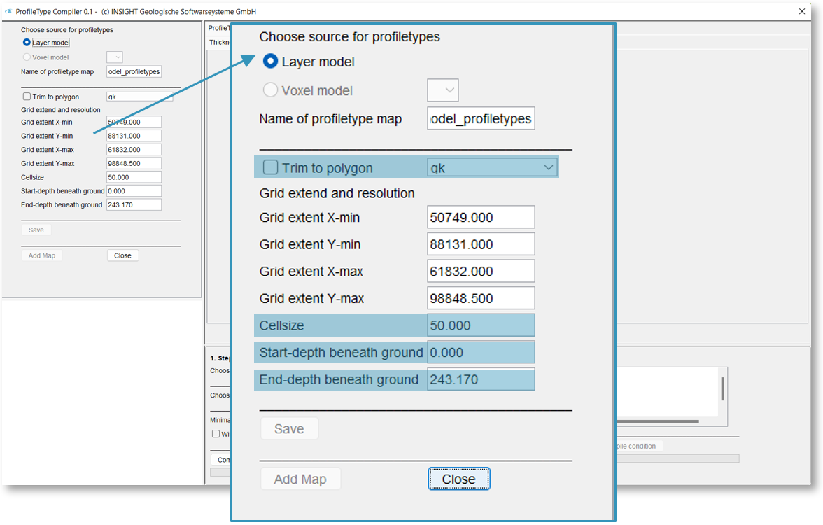
On the left side you select from which source the profile types should be calculated (for the voxel or layer model). The profile types are determined with a grid. At each node, the layer structure is compared with the other grid nodes and the same layer stacks are combined into one profile type. The cell size of the grid used and how many nodes are considered can be adjusted under Cellsize. The maximum depth at which the layers are recorded can be determined in the fields Start depth/End depth beneath ground.
If there is an area polygon in the model, e.g. a water catchment area, the profile types can be created for this area with Trim to polygon.
¶ Profile type maps for layer model

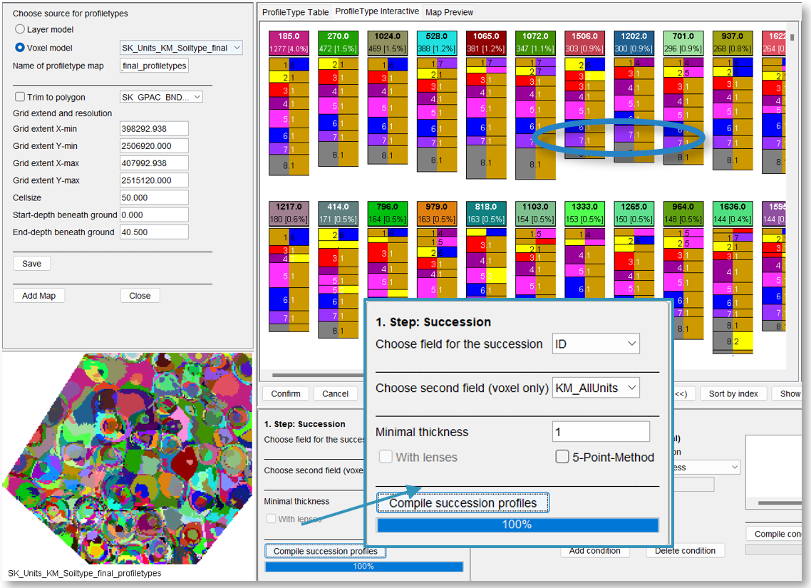
In the lower part of the window under 1st Step: Succession are the tool Compile succession profiles. It is used to calculate the profile types. After selecting this tool, you have to wait until the profile type map has loaded. On the left side you can see the settings for the grid and in the large area on the right the profile type table.
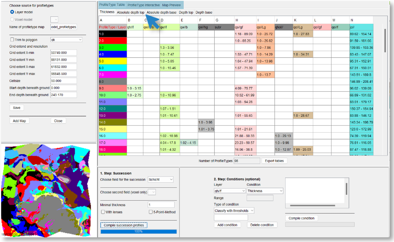
There are three tabs in the top tab. To enlarge the map, which can be seen at the bottom left, the tab Map Preview is opened. A legend can be found under the tab "Profile Type Table". In column A the profile types are numbered in ascending order and marked with a colour. One line describes the structure of a profile type. Each additional column represents a layer. As soon as a value for a certain layer is contained in the table, the profile type contains this layer. The values within the table show the thickness of the layer summarised in the profile type in the screenshot. In further table sheets are the specifications for Absolute depth top, *Absolute depth bas, Depth Top and Depth Base.
Note:
Absolute Depth is the absolute height starting from sealevel and Depth is the relative height from the lower and upper edge of the terrain.
Depth is the relative height from the lower and upper edge of the terrain.
Below the table is an indication of the number of profile types and the Export Table tool, which is used to save the five tables as a DAT file.

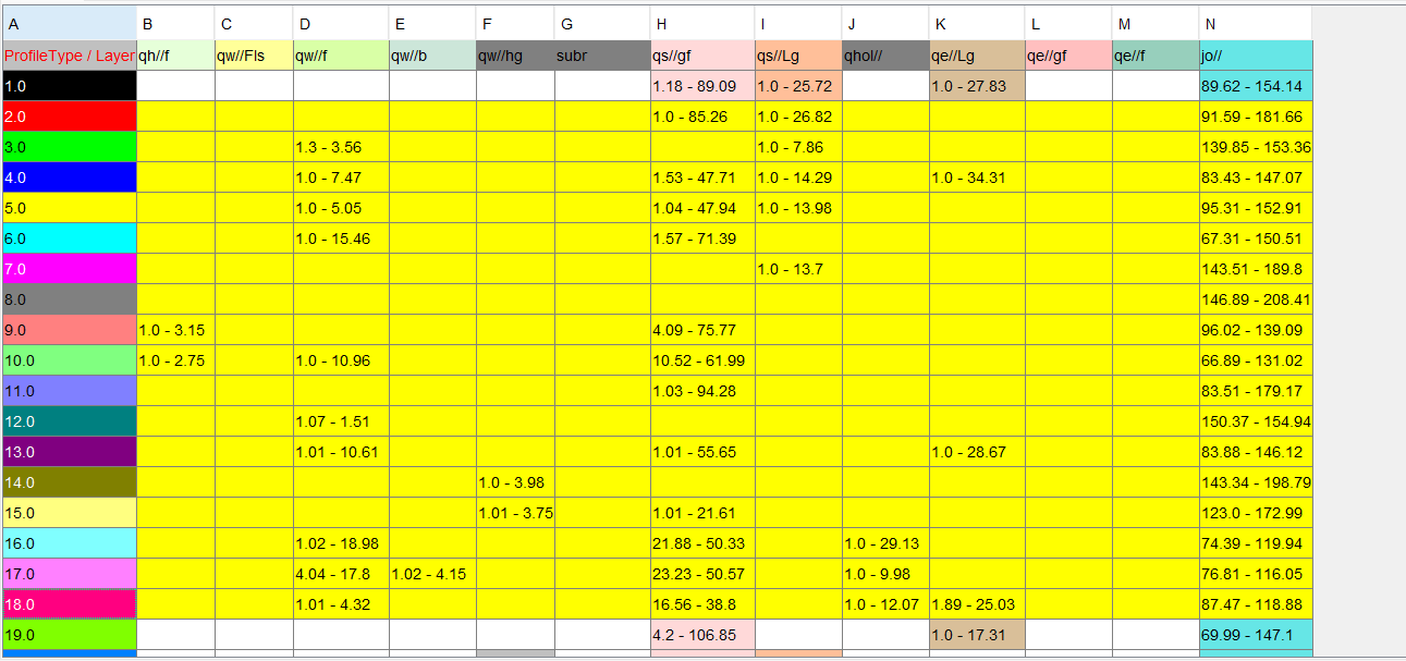
If a row is selected, the area of this profile type is visible separately in the lower left screen and the cell row is highlighted. In the tab Profile Type Interactive the profile type is displayed. Under this tab, a graphical representation of the layers that overlie each other in the corresponding profile type is shown. A selection of several profile types can be determined, which are to be viewed both in the map and in the interactive view. To do this, several rows must be selected in the Profile Type Table with the Shift key. To select another cell, the Ctrl key must be held down while clicking. In the lower left window, the number of grid cells filled by the profile types is indicated.

The quantity of certain profile types in the area can be recognised. It is decided whether these could be combined with a similar profile type that occurs more frequently. You can read more about this below.
In the Profile Type Interactive tab, sorting of the profile types and a graphical overview is possible. In addition, it can be seen how many cells from the grid are occupied with this profile type. This value and its relative percentage can be read below the index. The information depends on the accuracy of the model according to the information on the size of the cells in the grid.
¶ Sorting and summarising profile type maps
Below, the layers are shown with their name, colour and their relation of thickness to each other. The order in which the profile types are created can be selected in the bar.

The selection options are Sort by cell count (>>) descending, Sort by cell count (<<) ascending and Sort by index for sorting according to the numbering of the profile types. The Show all button displays all profile types (including the unselected ones). An image of the stacked layers of profile types can be saved with Save image. The image of the profile types is saved as an svg file, this vector graphic can be opened via a browser or editing programme.
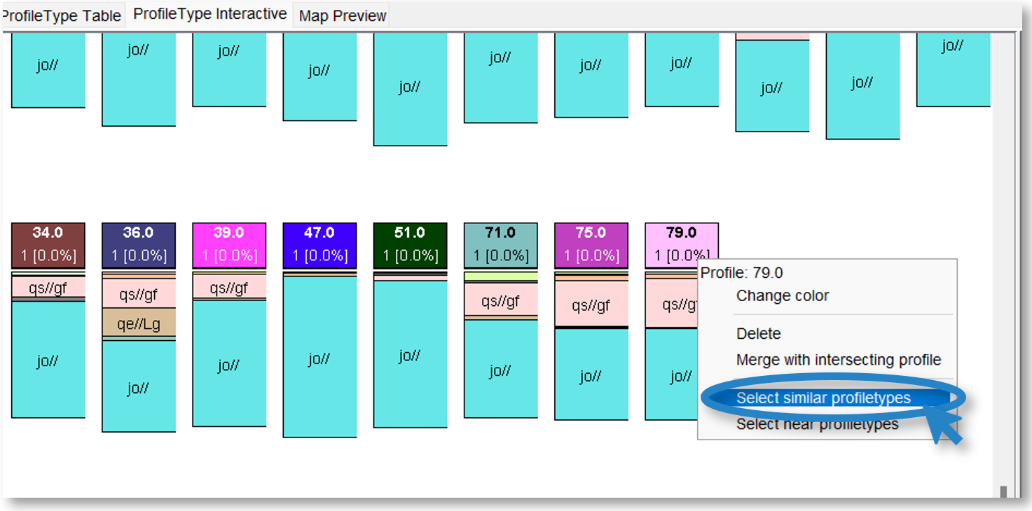
When the Profile Type Interactiv tab is revealed, the profile types can be sorted in descending order by their number of cells. There are profile types with very few cells. To reduce the number of profile types, right-click on the corresponding last profile type. With Select similar profiltypes the selected type is combined with a similar one.
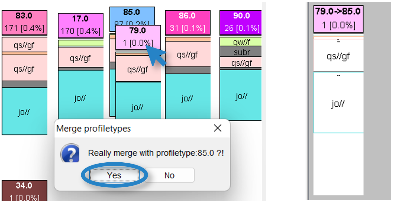
In this example, all similar profile types and the number 79, which is to be combined with another, are opening. A profile type is selected with which the 79 is to be merged. The mouse is held down to select profile type 79 and drag it into another. The process is completed with a right click and Merge and the confirmation Yes. The process can be seen on the right-hand side in the grey area. To undo the process, select it on the right and undo it with Recover.
With Confirm the whole operation is confirmed and you return to the profile type display with all profiles. In this way, the number of profile types can be reduced and classified.
Further options are opened with a right click. The colour of the profiles can be adjusted, a profile type can be deleted or near profiletypes can be displayed. In the latter case, profile types are displayed whose area is adjacent to that of the selected profile type. This can be shown in the map on the left.
¶ Set conditions for the profile types
In addition, conditions are set for the formation of the profiles, which can be defined below in the right field under Step 2: Conditions (optional). Accordingly, a choice can be made among all layers and the set of values and a minimum or maximum value can be selected or the threshold values can be classified.
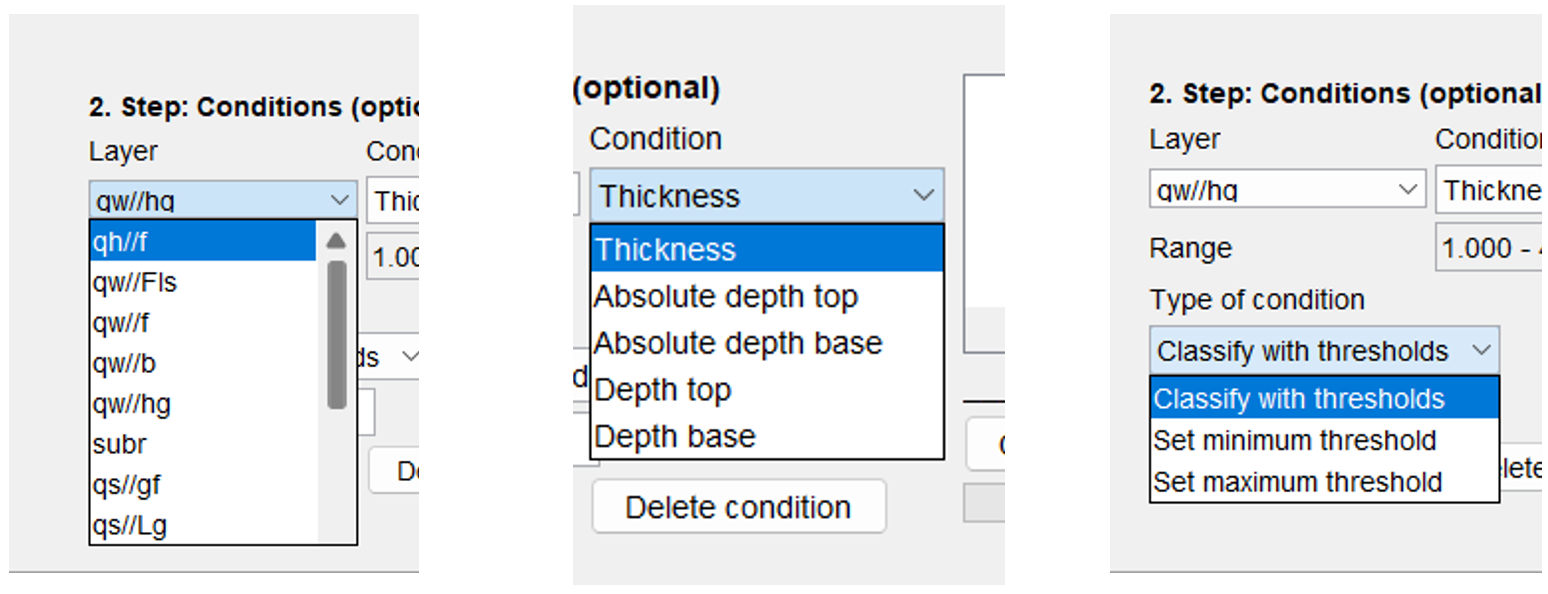
Under Add condition, further conditions can be added or confirmed with Compile condition. If a condition is to be removed, the condition is selected in the white box on the right and deleted with Delete condition.

After adding the profile type map to the model, it is displayed in the 2D map view as a new map under GeofactorGroup.
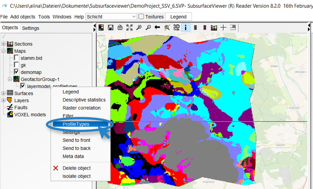
If this profile map is clicked with the Info Tool, the profile types are displayed at the coordinate with thickness, depth etc. The entire profile type table and map can be opened by right-clicking on the geofactor under "Profile Types". No more editing is possible except for the sorting function and hiding or showing profile types.
¶ Profile types for voxel model
If a voxel model is available, the profile types can be calculated based on the voxel. Two factors can be selected in "Step 1: Succession", as in this example model (ID and KM All Units). Otherwise, the settings for area size and cell size are the same as for the layer model and can be set before the calculation with Compile succession profile. Under Profile Type Interative the column is split into two values. This is created by combining the profile types with two parameters at the same time. This results in a variety of different profile types. The value used for calculation is in the middle of a cell. With the 5 Point Method, not only the centre is calculated, but also the nodes, in order to get an average value from all points.
¶ Spatial Multi-Criteria Analysis
Under the menu field Tools is the option Spatial Mulit-Criteria Analysis (SMCA). With this assessment function, a variety of environmental, social and economic data can be identified with a logical process for different factors. The site assessment can be carried out with several criteria at the same time.
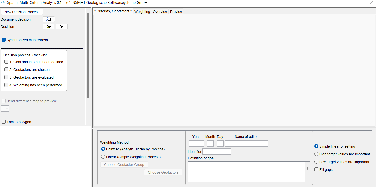
When the SMCA window is open, a new decision process can be started. Alternatively, files can be uploaded with the tool at the top left  where a process has already been started. This can be saved as an XML file
  or opened again. The decision-making process can be recorded as a document
  to trace the decision-making process. If a process has been started, with New Decision Process, all previous processes can be deleted and started again. A window appears with a warning that the information will be lost, this must be confirmed before starting.
With a tick in Synchronised map refresh, the map, which can be seen at the bottom left, will adapt to the decisions. If processes take too long to refresh, synchronisation can be turned off.
On the right hand side is a tabbed menu at the top with the tabs Criterias, Geofactors, Weighting, Overview and Preview. The Preview item hides the map with the results. The remaining tabs are examined in more detail below.
-
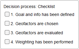 To create a decision-making process, use the checklist on the left side of the window as a guide.
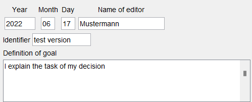 At the beginning of the process, an aim, date and editor of the process must be set in the field at the bottom in the middle. A keyword for the description is entered under Identifier. This will appear later on the process screen. When all the information has been entered, a blue tick appears next to Goal and info has been defined.
 -
In the lower field next to the goal and information, the geofactors are selected. Under Select Geofacorgroup the geofactor group from the model is selected for which the decision is made.
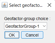
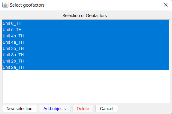
Under Select Geofactors, a selection can be made among the individual geofactors with the Ctrl key.
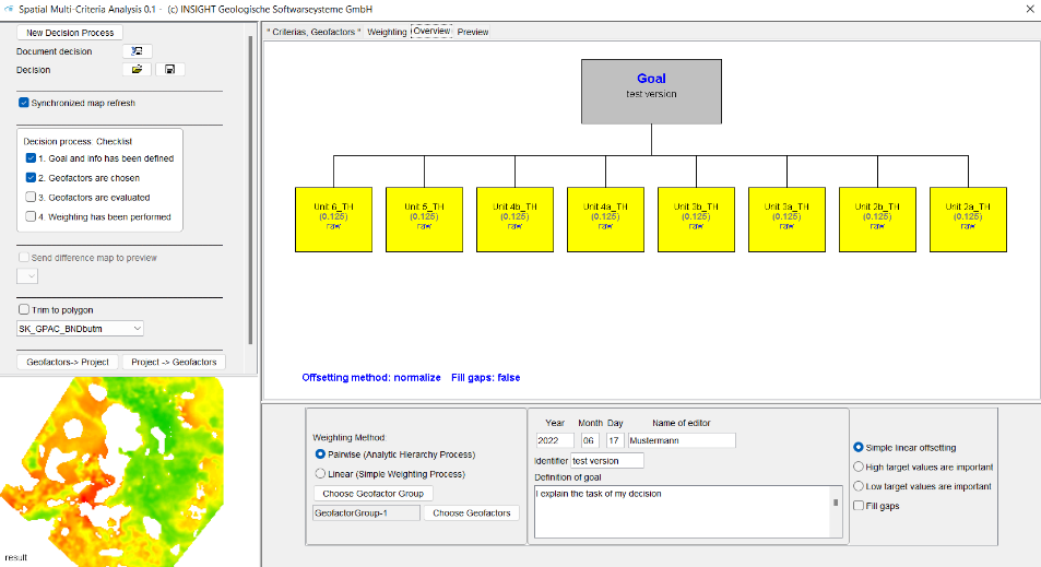
With New Selection the selection is confirmed. Geofactors can be added or deleted. A view of the geofactors appears under the Overview tab, which can be selected from the tab menu at the top. You can see a diagram tree with two levels. The lower yellow boxes are the geofactors that have been rated equally so far. After the geofactors have been selected, the evaluation can be started. To do this, the tabs with the geofactors are selected and, as with the geofactor (Geofactors), a target function is defined or the evaluation range is set. This must be done for all geofactors.
-
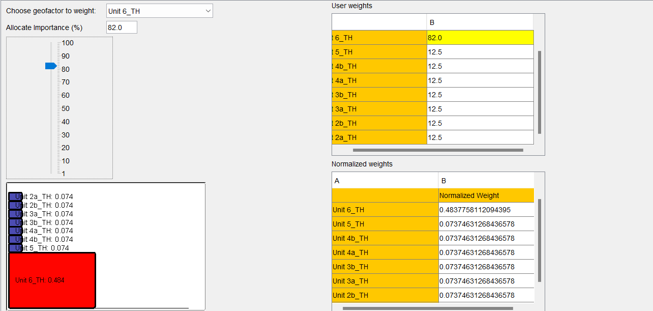 To weight the geofactors, click on the "Weighting" tab. The default setting for the weighting method (bottom left, above the button for geofactor selection) is Pairwise. This is the analytical hierarchy process according to Saaty (AHP). The Singel Weighting Process is set to Linear. First, one or two geofactors can be selected from the drop-down list at the top and compared or weighted linearly. This is done via the sliders below the selected geofactors. On the right side there are two tables. The first shows the User weight matrix and the second the Normalised weight matrix. The columns can be made larger or smaller by dragging the mouse along the edge of the column.
If the linear method was chosen, the individual factors can be selected and weighted. In the picture below with the rectangles you can see that their size adapts to the weighting and that the preview map has changed. The Pairwise method works in the same way. With this method, you should check under Consistency approved whether the weighting has not yet been accepted. In this case, a logical inconsistency was detected during the pairwise evaluation. The value to the right can be read off and used to adjust the rating.' -
At the bottom of the Overview, next to the graphical summary, is the rating in blue letters. The "Offsetting method" (you choose between "simple linear offsetting", "High" or "Low target value is important".) and "Fill gaps" can be seen. The gaps on the map, as shown in the bottom left of the screenshot, have been filled with data.
If high or low target was selected, the data is normalised by means of value maximum or value minimum. The optimal value, i.e. either the smallest (low) or the highest (high), appears in the result grid as 1. All other values evolve away from the optimum. This application is used on the primary search for the most optimal value of the real data. In the regular case, the setting is left at simple linear offsetting. All scores are normalised to the range of values between 0 and 1 using the settings and the objective functions and weighted together. After setting the weights under 3, they are offset linearly. All scores receive a low score for the worse condition and a higher score for the optimal condition. The result is a geofactor with score values between 0 (worst) and 1 (optimum). If there are gaps in certain grids and the assessment is to be completed with the other grids at this point, the use of the function Fill gaps is recommended. In doing so, the weights of the locally remaining geofactors are adjusted. If the function is not used, the system assumes that in the absence of geofactor information no evaluation can be made at this point. In this case, the result grid remains without an entry.
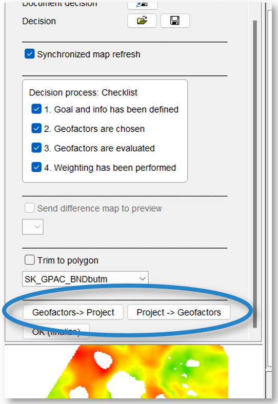
On the left side above the preview map is the option to adjust the geofactor grid to a polygon in the model. If one is selected there, the adjustment is displayed in the preview. In addition, the geofactor target functions can be transferred from target functions created in the project or vice versa. The metadata can be shwon in this window.
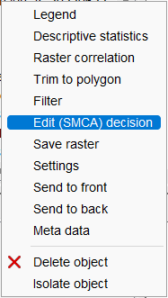 With *OK (finalize)* or the Save button at *Decision* the evaluation is implemented. A new object *SMCA-Result* appears in the model under which the geofactor grid is located. If further settings are to be made afterwards, right-click on the object to open the menu and select *Edit (SMCA) decision*. The SMCA window opens and the evaluation can be changed. With *Reset - last* or *Rest - initial* decisions can be undone.