Load geofactors in the Main Menu Bar under Add objects -> Geofactor-raster.
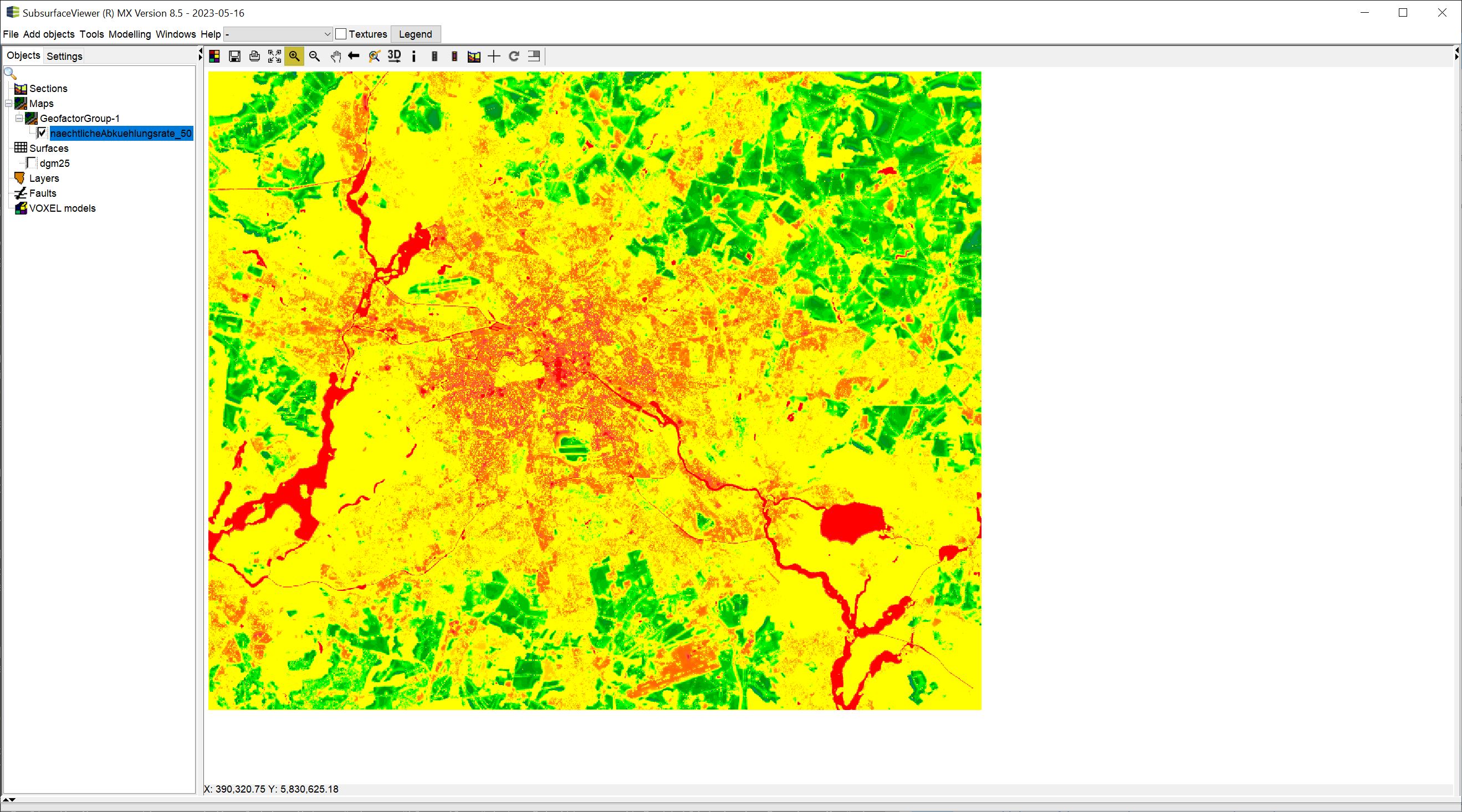
Note: The loaded geofactor is a downloaded grid from the FIS-Broker of the City of Berlin on the nightly cooling rate ("Umweltatlas Berlin / [Climate Model Berlin: Nightly Cooling Rate 2015 (Umweltatlas)]"). The evaluation that is carried out on this geofactor as an example is not a professional assessment. It does not originate from any scientific background and serves here only for presentation purposes of the functions of geofactors in the SubsurfaceViewer.
The geofactors are part of the implemented SMCA module (Spatial Multicriteria Analysis) (Multicriteria decision). In this article we will mainly deal with the specialised functions. This includes the evaluation tool. In the article Add objects you will find some explanations about the initial loading window without having Show evaluation active.
The possible formats for loading geofactors are listed here.
A loaded geofactor appears under the category Maps in the 2D-View object tree. Geofactors are assigned to automatic subfolders based on their extent and resolution. You cannot move these, as they are needed when creating a multi_criteria_decision.
¶ General Options
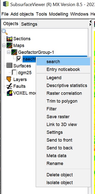
Open the options and functions for geofactors by right-clicking on the object in the 2D-View object tree.
The general options, which are assigned to other objects in the SubsurfaceViewer, can be found under Objects/Settings.
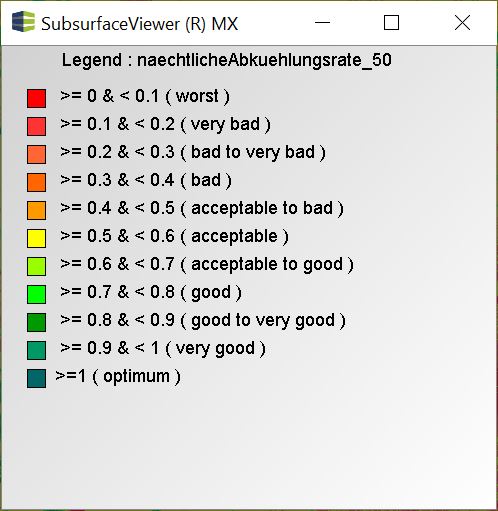
Legend: The legend shows the currently loaded legend defined in the Settings.
Descriptive statistics: This option displays graphics and information on the descriptive statistics of the (currently transformed) raster.
Raster correlation: This function is reserved exclusively for geofactors. Therefore, we will go into it in more detail below.
Trim to polygon: Filters the raster data based on a polygon copied into the buffer, such as a layer boundary or the boundary of a particular viewing area.
Filter: This is the filter we have implemented for all 2D and 3D raster data as well as parameters. As it deserves a more detailed explanation, we refer you here to this article.
Save raster: This saves the raster in its current transformed and/or filtered state. The dimension is always included, even if the data space has been reduced by filtering. If you have neither transformed nor filtered, use this to create a copy of the geofactor.
The Settings are discussed in a separate subchapter.
¶ Raster correlation
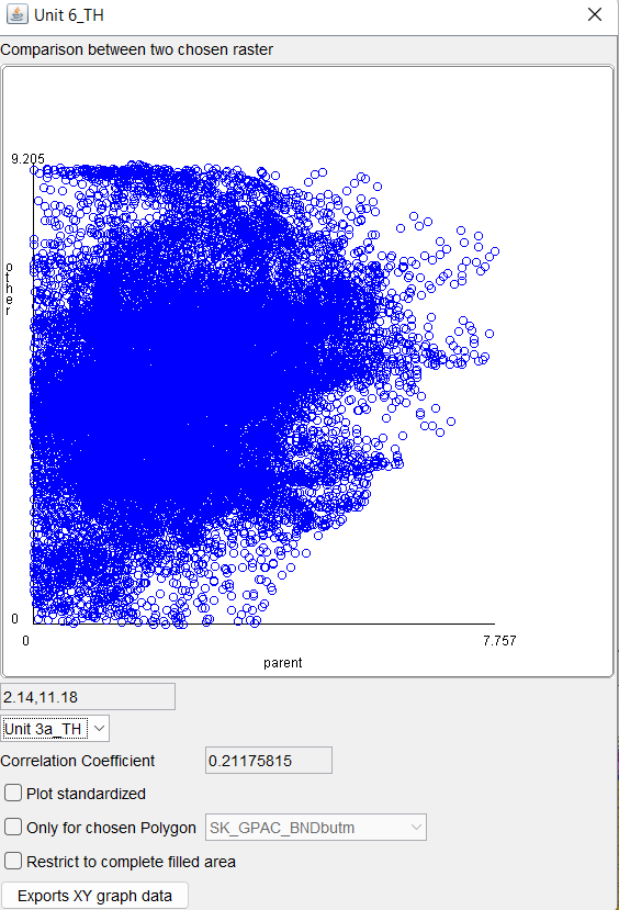
The Raster correlation can be found under geofactors. Use this tool to check a possible correlation between two raster data sets. You get a graphical representation of the value pairs in a 2D plot and the Pearson correlation coefficient is calculated with different settings.
Important note:
You can use the Raster correlation tool with geofactors of the same subfolder, i.e. of the same dimension and resolution! {.is-warning}
Centrally, the 2D plot of the two raster data in relation to each other in the form of a scatterplot is shown. The value scale on the X and Y axes corresponds to the value range of the two rasters.
Below the graph is a small coordinate text box that updates when you move the mouse over it, to help you analyse the data.
Below is a dropdown list. All geofactors of the same subfolder are listed. Select the geofactor that is to be compared with it.
Below this is the field for the Correlation coefficient - the result of the calculation according to Pearson as a number.
With Plot standardised you show the scale of the graph for the standardised data set (z-score) of both grids.
With Only for chosen Polygon you can restrict the correlation in one or more selected polygon(s) of a Polygon Shape Object.
If you check Restrict to complete filled area, the calculation of the mean and standard deviation for standardisation of the two rasters is allowed with data that contain data at an XY location in both geofactors, i.e. do not have a NoData value at the location. Otherwise the standardisation is done with the mean and standard deviation of the complete raster data.
With Exports XY graph data you export the values of the two geofactor rasters into a table with two columns for the data pairs.
¶ Settings
In the article Add objects you will find explanations about the initial loading window without Show evaluation active. Concentrate on the field that opens when you check Show evaluation.
Note: Evaluations for geofactors in SubsurfaceViewer have a value scale between 0 and 1 in the result. 0 is the worst case and 1 the best case - the optimum. All other cases lie at certain intervals in between, depending on how many score levels you introduce.
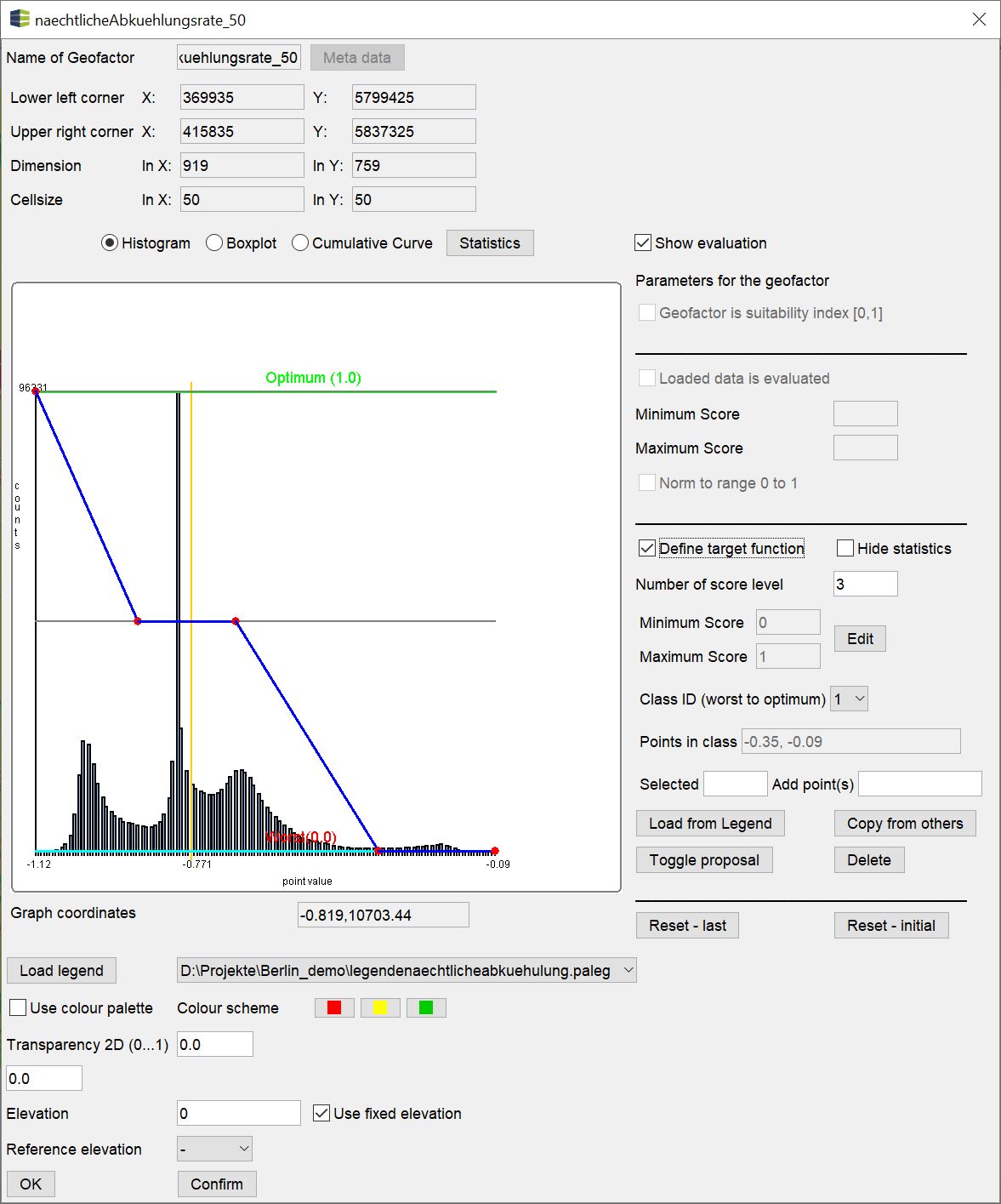
¶ Geofactor is suitability index [0,1]
This field is active if you have a geofactor as a result from the [SMCA tool](/en/Auswertung/Multikriterielle_Entscheidung). A tick is set there. The system has recognised the source of this geofactor. All other tick boxes with which you could make an evaluation are inactive. A decision should not go into an assessment again because it is itself already an assessment based on many criteria.
¶ Loaded data is evaluated
This field is active if you have not put a tick somewhere else on this page. By doing so, you define that this geofactor is already a result of a rating from outside. You have loaded a rated geofactor. Since a rating scale from outside does not necessarily lie in the value range between 0 and 1, but was perhaps carried out with integers between 1 and 10, you can enter the end elements for the worst and the best case for Minimum Score and Maximum Score respectively.
Caution:
Here you need to observe the following rules:The external evaluation must have been done with regularly distributed score levels - e.g. an integer assignment (1=bad, 2=medium, 3=good).
The small values must correspond to a poor score and the large values to a good score.
The minimum score and maximum score must be given on the basis of the rating scale that was used and not on the basis of the minimum and maximum entries of the grid. This is because a rating does not necessarily contain the worst or best case.
If you have a grid that fulfils the conditions contained in the info box above and contains the minimum and maximum score of the assessment, you can scale min-max. This is done with a tick at Norm to range 0 to 1.
¶ Define target function
If you check this box, you define a target function for this geofactor.
The view of the statistical plots should help to keep an eye on the data. You can hide them with Hide statistics. Then you will see the target function. If you switch between the types of statistical plots, you will notice that the objective function is visible everywhere. In the case of the box plot, it is of rotated by 90°.
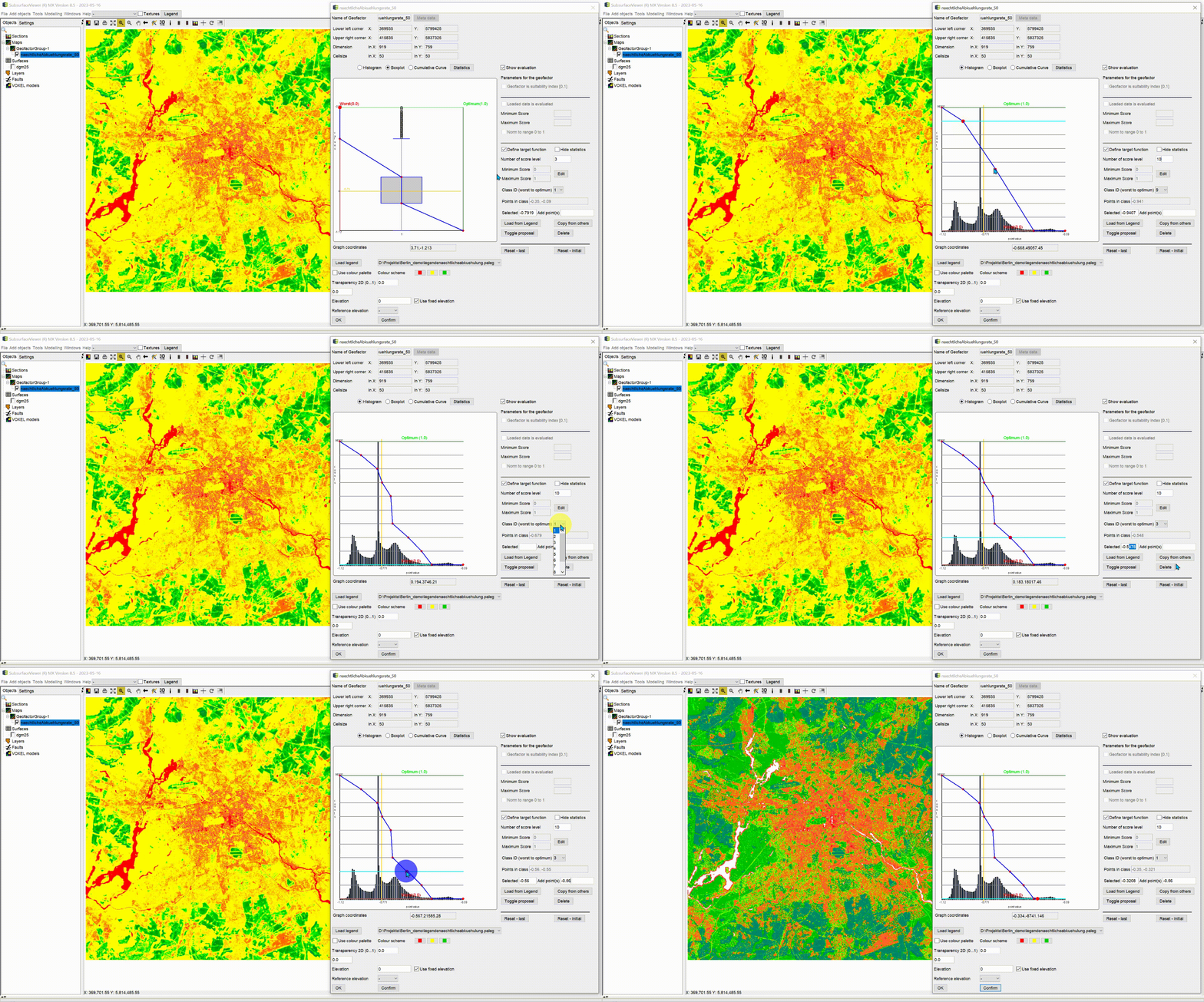
**A target function in SubsurfaceViewer is composed of any number of linear segments.
It is selectable in its form, theoretically it can be bell-shaped, stepped, jagged or similar. It can exceed or fall below the value range of the geofactor. Have a look at the example.
You can either:
- interactively directly in the field of the statistics plot,
- enter it directly,
- load it by legend,
- transfer it from other geofactors that have already been evaluated
- or generate it from a proposal.
The interactive option:
- Enter the number of regularly distributed score levels in Number of score level. You do not have to assign concrete limit values to all levels (score levels). But the scale should have a corresponding number of levels, depending on the planned complexity of your objective function, because at the levels you can enter "breakpoints" or "fixed points" as limit values for the score level.
- Go into the graphic with the mouse.
With a double click you and set a fixed point. This is automatically "snapped" to the nearest step to your mouse. You can "grab" this point with the mouse and move it further. Note that you cannot move the fixed point of a limit value beyond the next higher limit value, i.e. to the right. The points on the evaluation levels may leave the value range of the geofactor. Similarly, if the point is shifted to the left to lower limit values. If the previously lower limit value is thereby undershot, it is immediately adjusted to the lower value. You would get the same limit value at different levels. This makes sense if you want to see a "hard" classification without linear transitions. The lines between the levels appear vertical (histogram view). The exact limit value in a "hard" classification receives the rating level in the following to the right. If the transitions from one level to the next are not occupied by exactly the same limit values, the lines between them appear diagonally. When transforming the geofactor into the rating, a linear interpolation between the rating levels will take place on the values of the geofactor that lie in the interval of the two limit values. Generate objective functions with linear "soft" transitions between the valuation levels, as we show in the example. Fixed points that have both the same level and the same limit value are reduced to 1. I.e. you do not need to worry about duplicates.
If you want to delete a fixed point, right-click on the "fixed point" and it will disappear.
If you now want to enter an exact limit value for a fixed point that you have set interactively, select it with a mouse click and enter the exact limit value in the field at Selected. The fixed point updates its position as soon as you have confirmed it in the field with ENTER.
Via direct Input:
- Enter the number of regularly distributed score levels in Number of score level. You do not have to assign exact limit values to all levels (score levels). The scale should have a corresponding number of levels, depending on the planned complexity of your objective function, because at the levels you enter "breakpoints" or "fixed points" as limit values for the score level.
- At Class ID (worst to optimum) is a dropdown list with integers - as many as you have defined rating levels. Use this dropdown list to skip back and forth between the rating levels. Level 1 corresponds to the worst case. The active rating level is shown in turquoise in the graph. At Points in class shows a list of the limit values which are set at this level. If you want to manually enter a point on the currently active evaluation level, write the limit value in the field Add point(s). If you want to position several limit values, enter them comma-separated. As soon as you confirm in the field with ENTER, the point is added.
Note: Enter the fixed points in the order of the limit values from low to high (in the histogram on the x-axis from left to right) to avoid strange effects of the objective function.
Note: To present an interactive objective function, select the values and set them to exact limit values, is the quickest option.
Via a legend:
Here you can load a legend in *.beleg or *.paleg format. Have a look at the formats here. You can create a legend with the legend-editor. You can save a legend outside, and thus it can be useful for a documentation of the target function. You can use this to make "hard" classifications, i.e. staircase-like objective functions without linear transitions between the evaluation levels.
Via other geofactors:
If you have geofactors in the project which should have the same objective function, you can select the corresponding one with Copy from others.
Via the proposal
Get a proposal for a target function with the button Toggle proposal. These objective functions are based on robust descriptive statistics. Turn on the boxplot and press the button several times to see it. Various combinations of minimum, maximum, median, interquartile range and limits of mild outliers are formed as objective functions.
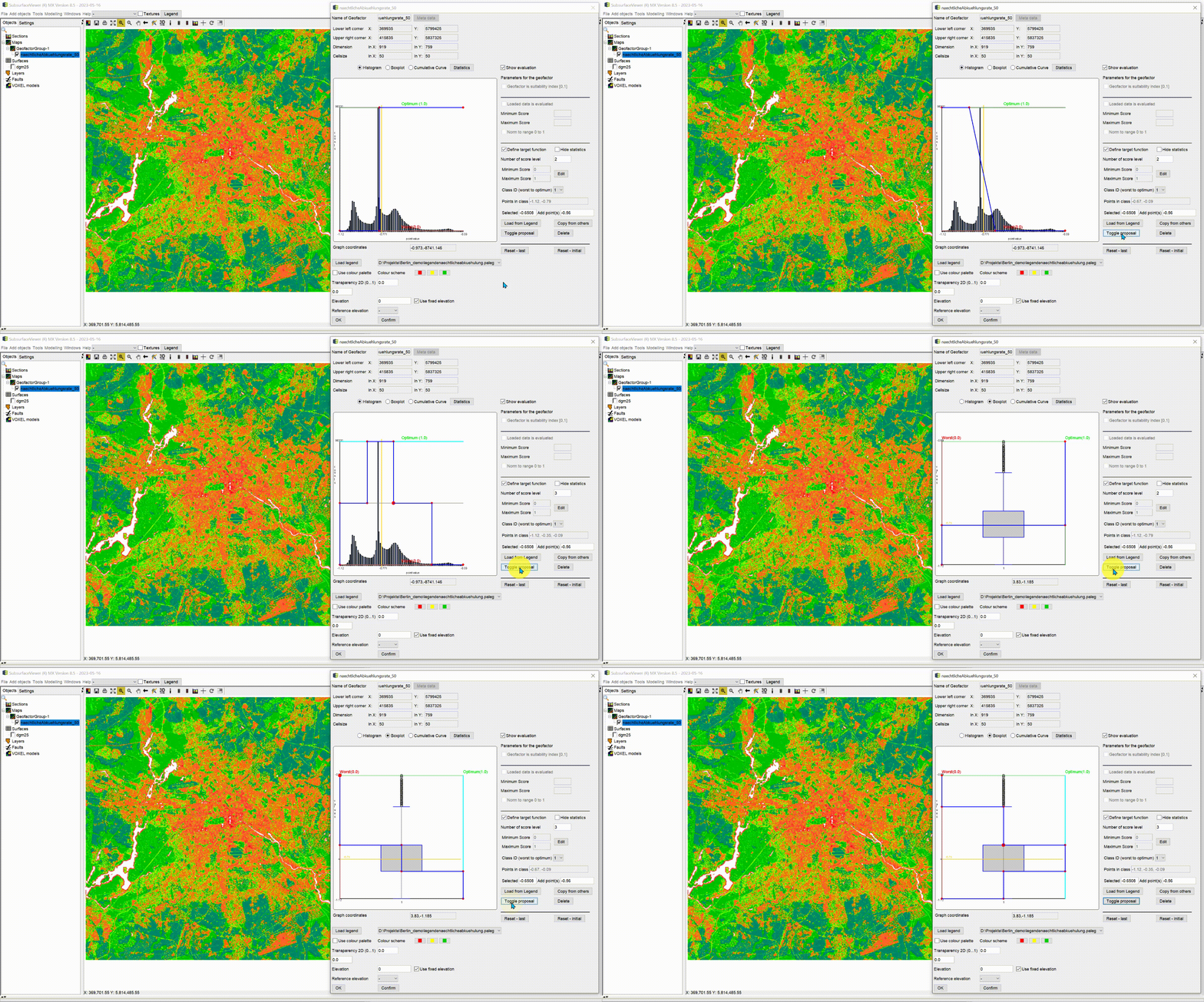
Always confirm a transformation of the data, based on the target function or the other methods via Confirm or OK.
The edited geofactor raster in the 2D-View shows the transformed values (between 0 and 1). You can export the raster with Save raster if you want to use it elsewhere.
Note: If you want to exclude the highest or lowest values of the geofactor from the evaluation, shorten the objective function by moving the fixed points of the last limit members into the value range. All raster values that are no longer covered by the target function are set to a NoData value in the transformation.
With Delete you delete a set target function and start again.
With Reset - last you jump back to the evaluation that was last confirmed.
With Reset - initial you get to the settings of the evaluation that may have set when you reloaded the saved project.
Tip: If you want to use the functionalities of the target function determination, but the output grid is to be migrated to another programme, and you do not like the value range 0-1 for the output grid, press the Edit button under the Number of score level field. The fields Minimum Score and Maximum Score will become active and you can e.g. enter integers from 1 to x to get a different range of values.
