**The LogExplorer is part of the Parameter Manager. You should be familiar with the basic features of the Parameter Manager before tackling this tool. In addition, it is still noted with a beta status due to limited test phases. Please feel free to contact us if you have any questions or comments.
Open the LogExplorer via the Parameter Managers.

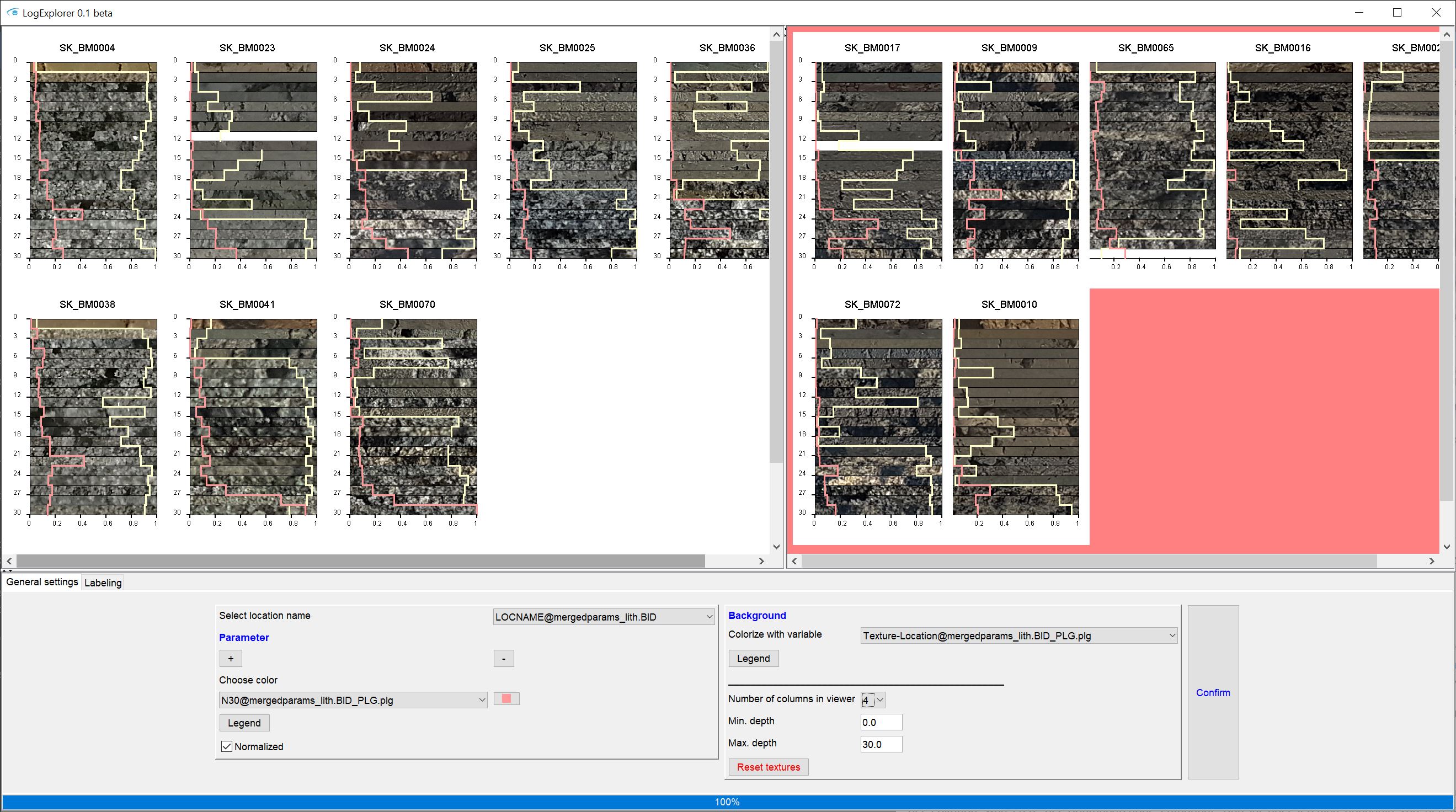
With LogExplorer you can display your downhole parameters from borehole measurements (e.g. pressure soundings), borehole descriptions (see parser for layer descriptions and SoilType-Tool as well as other punctual in-depth information as curves individually or together. You can additionally visualise texture tables from core samples as background of your parameter data at the drill point. We provide functions for manually grouping boreholes and manually labelling layer data. The LogExplorer is connected to the Data Tree and is inactive if you have not created one.
The LogExplorer is to be understood as supplementary to the profile section construction and the definition of layer lower edges of the correlation of layers. If the geological concept is uncertain, it can provide interim views, mark anomalies, combine different views of the features of a borehole measurement or description, and export tables for interpolation in SubsurfaceViewer or a third-party programme.
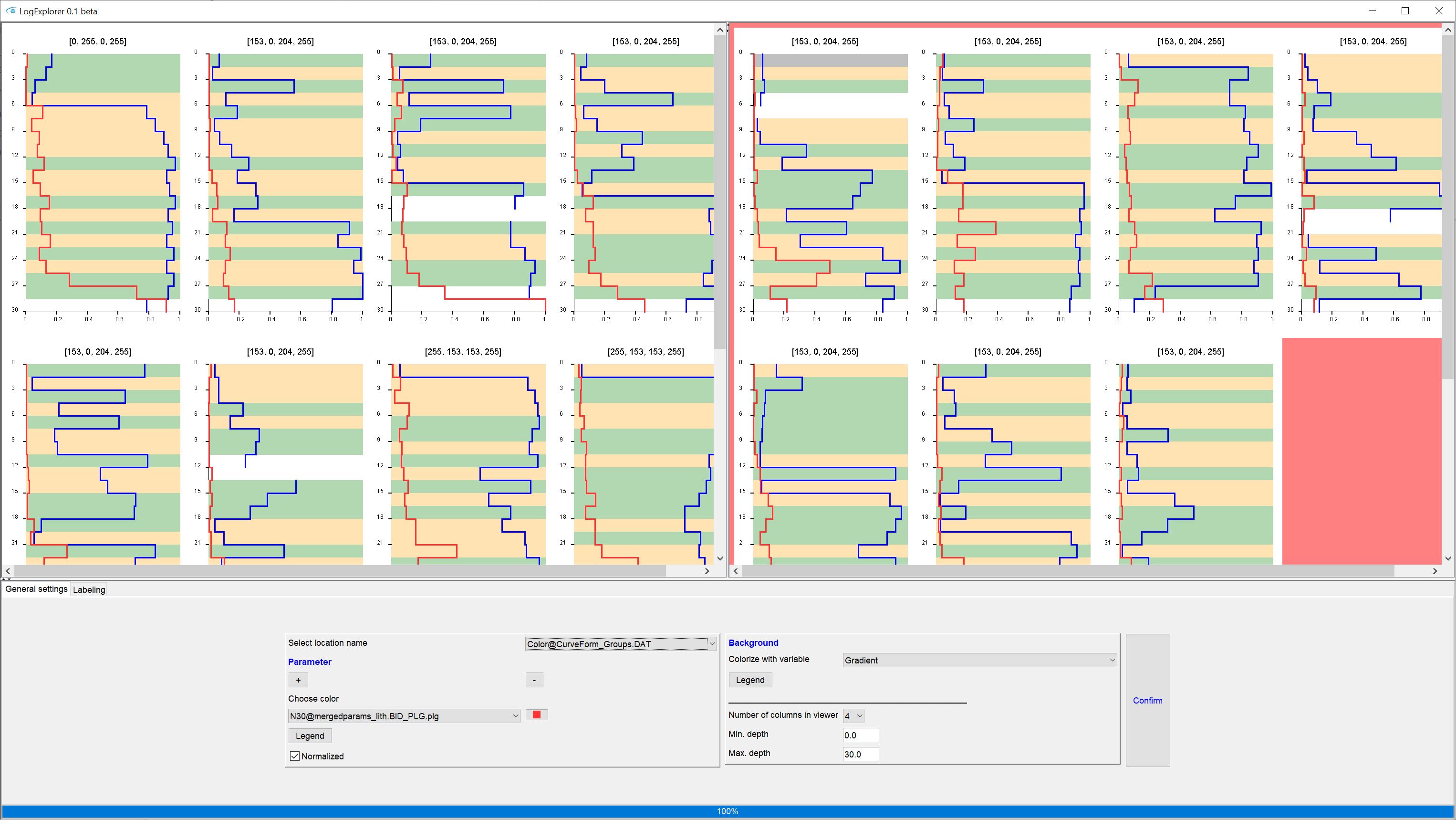
When you open LogExplorer for the first time, you will see a tripartite user interface. The large white boxes will fill up with your curve plots once you have made your settings.
At the bottom is the options bar. There are two tabs available: General settings and Labelling.
Under General Settings you define settings for the visualisation of the curve plots.
Under Labelling you will find options for manually grouping boreholes and labelling layers or horizons.
**If you have coupled the LogExplorer in the LocView object, the last clicked location will be moved into the view in both upper windows and framed in black. This way you can work synchronously with LogExplorer and the standard user interface of SubsurfaceViewer. We recommend working with at least two screens for this.
¶ Upper left window
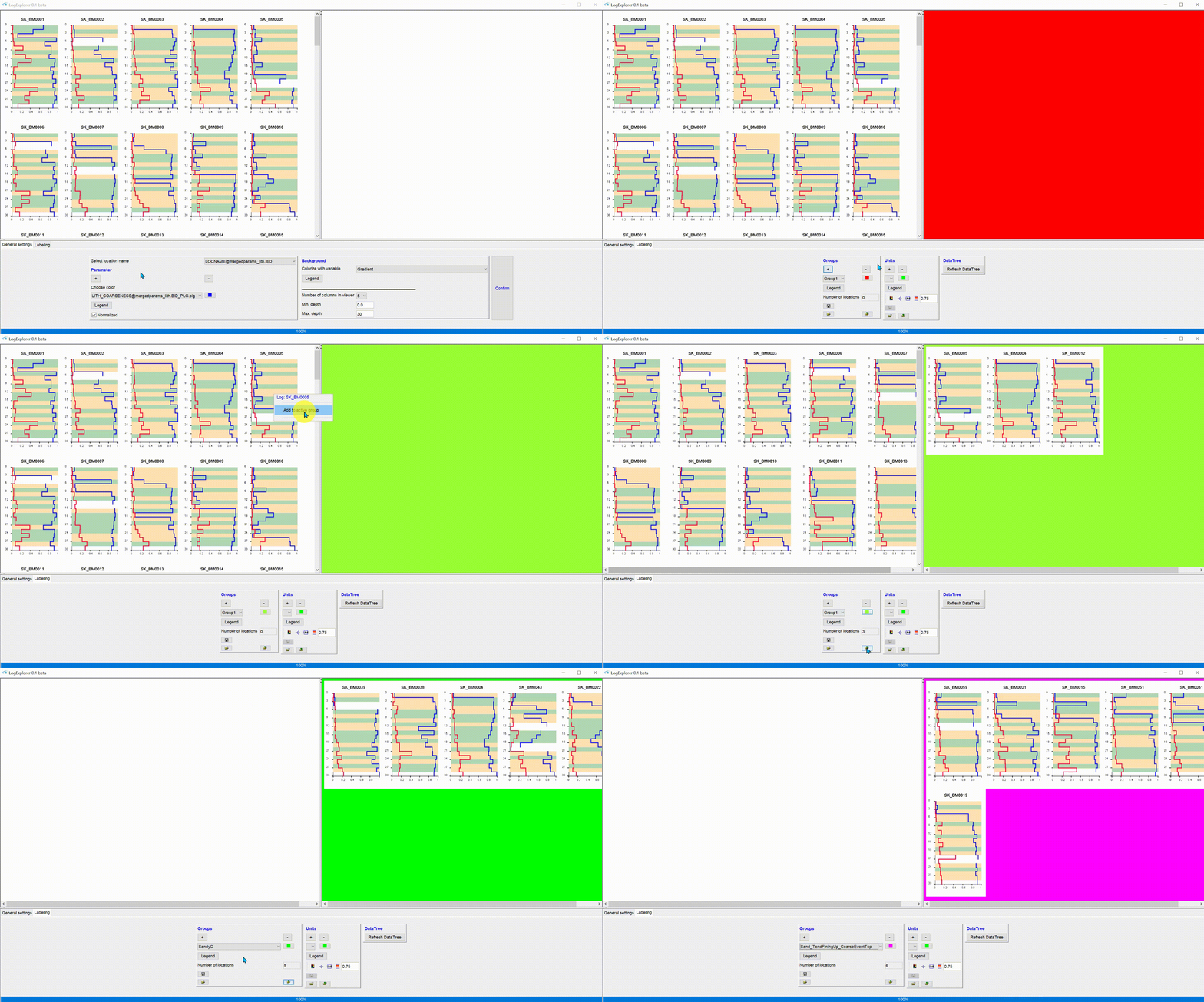
Here you see your curve plots as they are loaded ungrouped. I.e. all boreholes that have not (yet) been assigned to a specific group by you via the Grouping Tool are located here. You can assign curve plots to an active group from here via a right-click context menu. Read the section on grouping for this.
Note: The size of the upper left window is decisive for the aspect ratios of the individual curve plots. If you want to see wider figures, move this window further to the right; then vice versa for narrower curves.
As long as you do not have the layer labelling tool active, each curve plot is freely movable by drag&drop using the left mouse button. The view will not be re-sorted until you reload the Plots. We have made these plots movable so you can compare curves at different locations more easily. Therefore, move the corresponding images next to each other.
¶ Upper right window
You can see your curve plots as they were grouped by you. The group currently active in the grouping tool is shown, which you can also recognise from the background colouring. Read the section on grouping for more information.
Note: The size of the upper left window is decisive for the aspect ratios of the individual curve plots. The curve plots are displayed in the right window with the same number in a row as on the left. If the right window is much narrower than the left window, the individual curve plot images may overlap in the right window. You can also move the individual images freely here and thus have the option of adapting the display for you once again.
¶ General Settings
Here you set the options for the display of the curve plots.
You can pass the location names to your curves in the title. As a rule, this will be the borehole name. If necessary, select other parameters, such as information from the metadata of the borehole or a grouping - depending on what you have loaded into the data tree. To do this, use the dropdown list that is displayed for set location name.
Numerical parameters that belong to the borehole are added with +. A small dialogue window opens in which the numerical parameters in the data tree are displayed. You can add one parameter at a time. Once you have confirmed the selection, the parameter name is added to the Dropdown list under Choose colours. You can set the colours for the corresponding curves by selecting the parameter in the list and editing the colour button. The window that opens when you press the Legend button shows an overview.
If you leave the tick under Normalised active, all parameters are min-max scaled, which means that your value range is always between 0 and 1. This makes it easier to visually examine parameters with different scales together. If you deactivate Normalised, the values are displayed as they are.
With - you delete the currently active parameter of the Dropdown list under Choose colours from the display.
Under Background you can set the background of the display. By default, this is set to Gradient. This background is used for an overview of the development of the primary parameter with the depth. The primary parameter is always the first parameter selected in the list. If you want to change it, you should delete all parameters and select them again in the correct order as described above. A pale green colouring corresponds to a decrease of the parameter in depth, or in relation to a lithological sequence, a coarsening up. The pale yellow colouring marks the opposite case, i.e. in relation to a lithological sequence, a fining up. A grey colouring informs that it was not possible to determine at the site whether it was an increase or decrease in depth. A white colour indicates a data gap.
.gif)
You can select another parameter for background colouring. The colouring is individually adjusted under Project View in Parameter Manager. If nothing is defined here, a standard legend is created. Open the legend for the parameter with the button Legend in the area Background for viewing.
Under Number of columns in viewer you determine the number of curve plots in a row using the Dropdown list. This refers to the upper left and right window. In combination with the size of the upper left window, this setting determines the aspect ratio and the size of the curve plots. Try it out to get the most favourable display for you.
Below you will find two text fields with the title Min. depth and Max. depth. Here you define the depth interval at which you want to view the curve plots.

If you have (/en/Funktionen/CoreTextures)loaded textures from the Core Textures Table Tool, the red button Reset textures appears. Since loading, scaling and cropping core textures can take some time depending on the data set, the generated image sections are buffered in the memory. This allows you to change curve colours without waiting for the textures to reload. If you change the size of the individual images when you create the plots, the cropping and scaling of the textures may no longer fit. Press this button to empty the buffer and trigger a new cropping of the images.
After you Confirmed your settings, the images of the curve plots are generated for each location.
¶ Labeling
Here you group boreholes or locations as a whole or label certain layers or horizons in depth intervals at the locations.
¶ Groups
 !
!
With + you add a group. A small dialogue opens in which you can specify a name for the group. After confirmation, it is immediately added to the dropdown list below. Use the Dropdown list to activate a group. You can see this in the upper right window by the background colouring. You can change the colouring with the button on the right of the dropdown list. The button Legend opens a window with which you can see all groups with their colours.
In the field Number of locations you can see the currently active number of locations that have been assigned to the active group.
Use - to delete the currently active group.
Save the result in a table with the extension *.dat.
It contains 6 columns: "LOCNAME" (as selected in the General Settings) + "X" + "Y" + "Z" + "Groupname" + "GroupColor". XYZ corresponds to the coordinates with the highest point at the location, which usually corresponds to the drill approach height. This depends on the data in the data tree. "Groupname" is certainly self-evident. "GroupColor" is the RGBA value in text array format, which is readable by the Parameter Manager for representations. This array can be used to load the grouping table with the same colour settings, or if you do not want to lose the information for third party programmes.
With the Open symbol you load a previously saved table in the same format as described above. The groups are created and the locations, are automatically assigned to the appropriate groups.
With the marked Open symbol you select a parameter directly from the Data tree for grouping. If necessary, an automatic legend can be created. This is usually loaded from the Project View setting of the Parameter Manager.
¶ Units
Here you create labels, i.e. markers for certain depth intervals at the locations.
 !
!
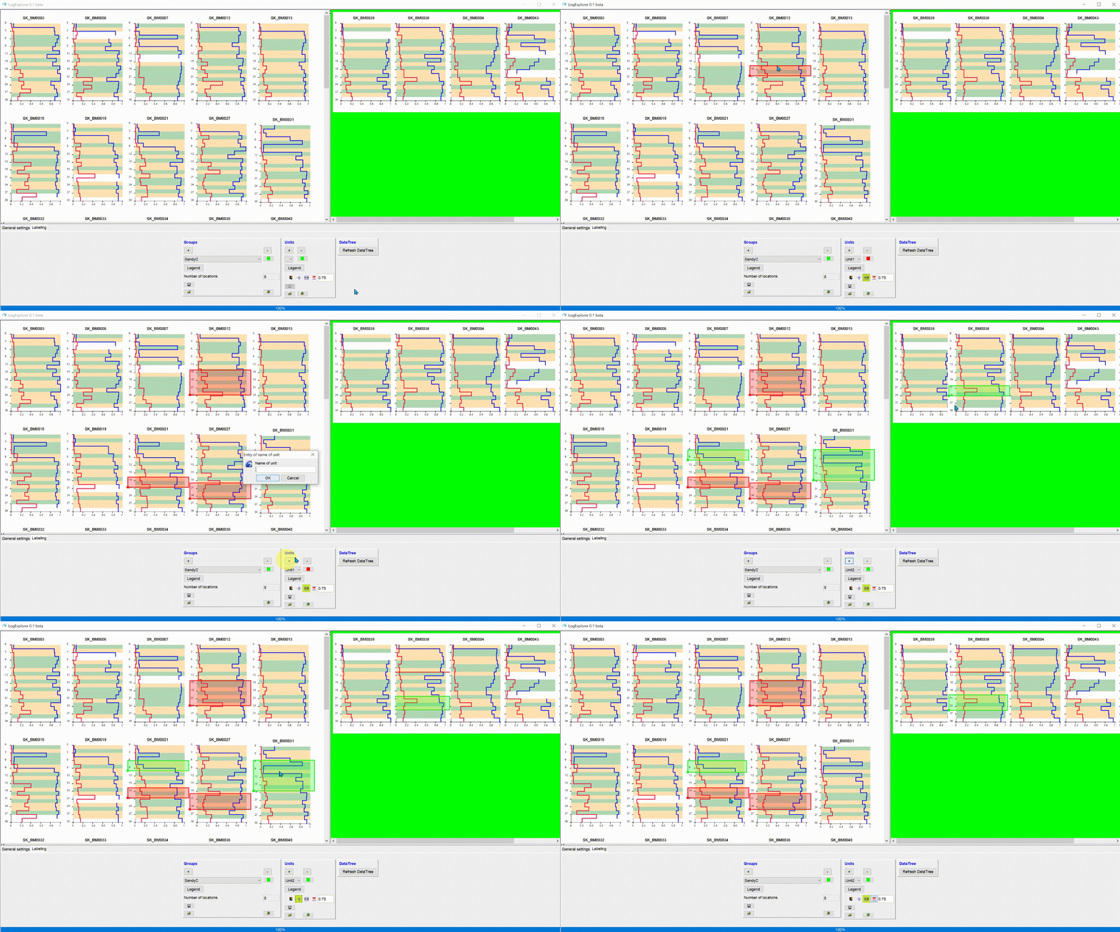
With + you add a unit or a marker. A small dialogue opens in which you can specify a name for the marker. After confirmation, it is added to the dropdown list below. Use the Dropdown list to activate this marker. You can change the colouring with the button on the right of the Dropdown list. The button Legend opens a window which shows the created markers and their colours.
Press - to delete the currently active marker.
Below the Legend button you will see a toolbar for creating markers/labels:
- Color chooser: This is used to set the colouring of guides.
- sequence line: Use this to create a guide line with the colouring defined above. Activate this tool by left-clicking with the mouse. You can no longer move all the pictures in the upper windows by drag&drop. Instead, you can place a horizontal line in a curve plot by double-clicking. You can drag and drop this line to the depth where you want to set the highlight. With right click on the line you get the option to delete the line. Note that this is only an auxiliary tool during your work. The lines are not considered when saving! If you deactivate this tool, all curve plots are free to move again.
- Unit: Here you enable the drawing of the active marker. Activate this tool by left-clicking with the mouse. You can not move all the pictures in the upper windows by drag&drop. If you deactivate this tool, all curve plots are free to move again. To draw a marker, double-click in the desired depth interval in the curve plot. A rectangle appears whose upper and lower edges correspond to the depth interval of the marker. By drag&drop directly in the rectangle you can move it up and down. If you click in the small square at the lower left corner of the rectangle and then drag it, you change the extension of the depth interval. With right click on the rectangle you can delete it. In addition, you can read the location name and the name of the clicked marker in the header of the context menu. This provides an overview.
4 Clip boundaries to sequences: With this tool you clip the depth intervals of the markers exactly to the nearest upper and lower edges of the primary parameter. There is a warning that there is no return for this.
5 Transparency: With the small text field you change the transparency value for the colour filling of the marker rectangles. A value of 1 corresponds to complete transparency and a value of 0 is opaque. If you already have several markers in the system, you will be asked whether you want to adopt this transparency value for all markers.
With the Save symbol you save the result in a table with the extension *.dat.
It contains 7 columns: "LOCNAME" (as selected in the General Settings) + "X" + "Y" + "Ztop" + "Zbase" + "Unit" + "UnitColor". XY corresponds to the coordinates of the location. "Ztop" and "Zbase" list the absolute heights (e.g. NN) of the depth intervals of the defined markers/labels/layers. "UnitColor" is the RGBA value in text array format, which is readable by the Parameter Manager for representations. This array is good for you if you want to load the marker table sometime with the same colour settings, or if you don't want to lose the information for third party programmes.
With the Open symbol you load a previously saved table in the same format as described above. The markers are created and automatically assigned to the locations, if they can be found.
With the marked Open symbol you select a parameter directly from the Data tree. An automatic legend can be created. This is usually loaded from the Project View setting of the Parameter Manager.
**Important note: Markers can only appear with one rectangle at a time at one location, i.e. if there are several markers/horizons with the same name at the same location in the data tree, a rectangle is created with the uppermost upper edge and the lowermost lower edge. If you create markers manually in the LogExplorer, you can delete a rectangle of the active marker by double-clicking to set a new one. We assume that a layer horizon or a marker horizon should only be assigned once at a location. This makes sense when working in unconsolidated sediments. We have not considered phenomena due to folds and faults at single locations here.
Tip: The rectangles of the markers may overlap. {.is-info}
¶ DataTree
When you press the Refresh DataTree button, you create the LogExplorer Grouping attibute in the data tree if you have created a grouping, and LogExplorer Units if you have created markers. You can evaluate these, with the Parameter Manager and also view them in the standard user interface of SubsurfaceViewer, e.g. in a section or in 3D. To do this, create a LocView object for the corresponding attribute. Let the linked article guide you.
Note: Don't forget to press the
Refresh button in the 3D view and in the Cross-Section window to see the current data tree status for the created labels. {.is-info}
!