Note: You will see a beta note in the title of the Parameter Manager window. The Parameter Manager has been developed on a project-specific basis, but contains many functions that can be used very flexibly. These could not yet be tested in their entirety. We have also made tools available whose basis was laid in the research project goCAM. We hope that by making them available to other users of SubsurfaceViewer, we will gain more experience in improving these functions. Therefore, please feel free to contact us to discuss this and possibly promote further development.
Important Note: Some of the functions implemented here use Python. It is easiest for you to allow the Python installation when you install SubsurfaceViewer. This guarantees the integration of all required libraries. In addition, you should have defined the python.exe path under Program Settings.
The Parameter Manager is used to integrate parameters into the visualisation options of the SubsurfaceViewer user interface (e.g. LocViewObject). In addition, it provides a variety of preprocessing options for a dataset, such as table linking, merging of data at the same locations, parsing for borehole descriptions, parameter analysis and advanced classification tools. Furthermore, advanced lithology analysis functions are integrated. We have compiled a practical example in the article Integrate Parameters.
Here you can find the explanations of the functionalities.
¶ The User Interface
The Parameter Manager can be found in the Main Menu Bar under Tools -> Advanced Tools -> For parameter.
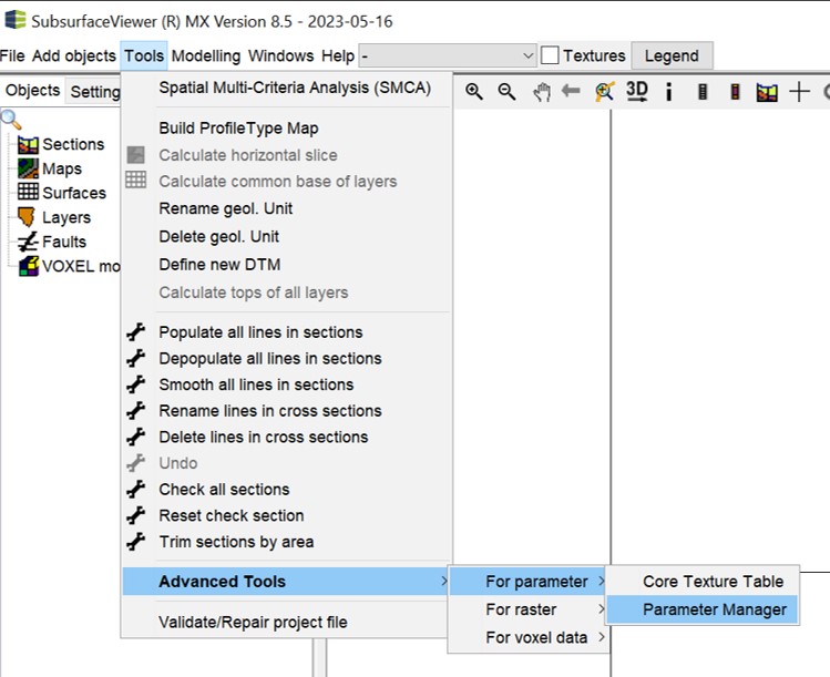
The shown window will open.
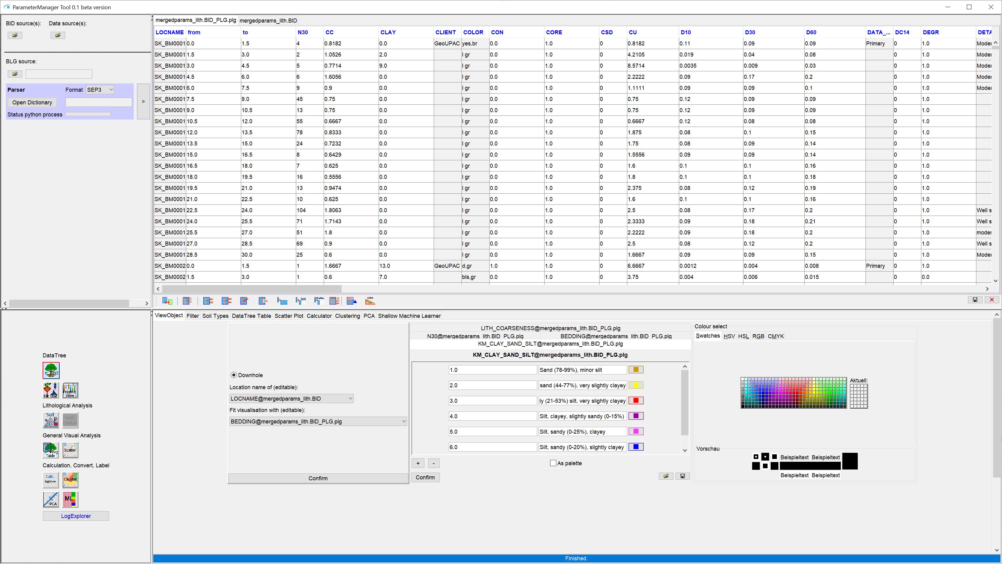
You can adjust the size of the individual window sections to your current activity by clicking on the bars and dragging them.
In the upper left section you will find options for loading tables in various formats. You will find the parser function for *.blg-files. Details on this are summarised for you in the section Load tables -> Parser for layer descriptions.
In the upper right window you will see the tables as soon as you have loaded them. Each table appears with its own tab, which you can also use to switch between the loaded tables. You have a toolbar at your disposal that offers you a variety of analysis and preprocessing options for your table(s). Details can be found in the section Working with Tables.
In the lower left section of the window you will see various buttons that allow you to perform advanced analysis, preprocessing and classification procedures. From here you prepare your parameters for visualisation in the Standard User Interface of the SubsurfaceViewer. Export functions in preparation for parameter interpolation with 3D-IDW and 3D-Kriging are also integrated. Some of the functions are not yet active unless you have created a data tree from your tables. You will find a summary of all these functions in the section Parameter functions.
The lower right window shows you the user interfaces of those functions that you have clicked on the left.
The Parameter Manager merges georeferenced data from tables in the so-called data tree (DataTree).
¶ Data tree
If you press the button DataTree ![]() in the lower left area, the data tree will be created.
in the lower left area, the data tree will be created.
Important:
The data tree is the most important basis for in-depth work with the Parameter Manager. If you don't want to "just" use a few functions on a table basis, you should create it, even if it takes some time for data-intensive table links (e.g. > 10 000 boreholes or > 500 000 point data).
You must have loaded georeferenced data from tables and, if necessary, linked to build the data tree.
Its structure is shown here symbolically.
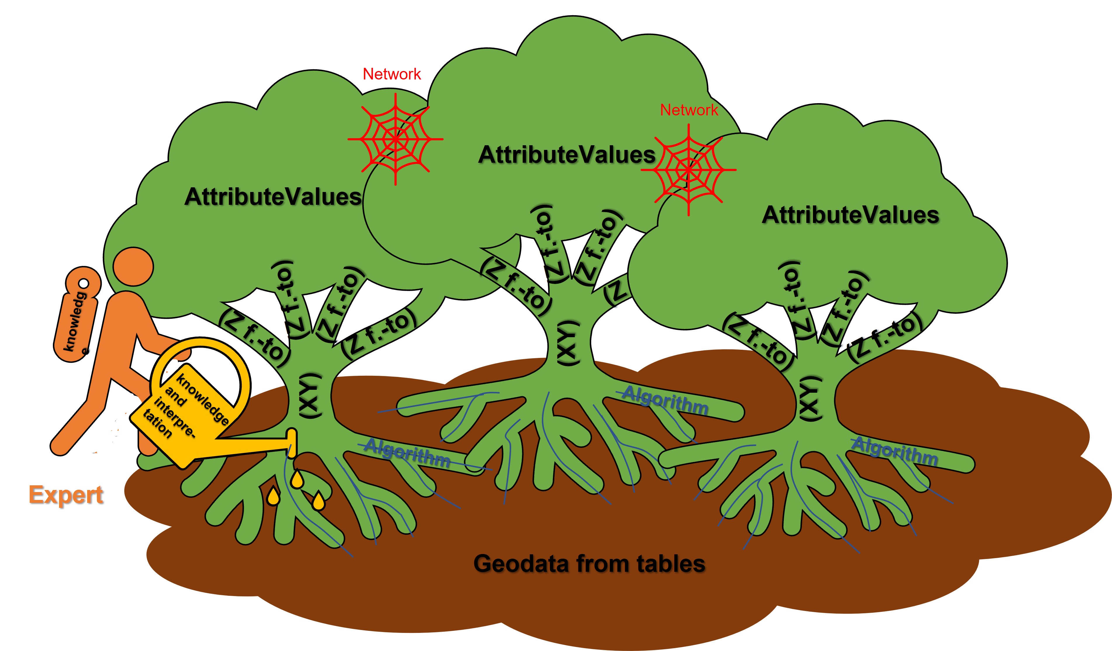
First of all, fluent coordinates are read from those columns of the loaded tables that define a spatial reference. You can read how to pass the spatial reference of the tables to the system here. So it is about X-, Y- and Z-coordinates, but also relative depths with a top and a base, as can happen for example with core samples.
The XY coordinates form the "main trunk" and the Z coordinates the "branches". All parameters that refer to these coordinates through your table links and the table location form the "leaves" of the data tree. They are combined into attributes, the "network", according to your column entries.
The attributes are given the name of the table header row in the corresponding column from which the parameter was read, followed by an "@" symbol, and behind it the short name of the source table. This ensures uniqueness in the case of the same column titles from different tables.
The fluid coordinates are only table references, like the parameter values. They are read directly from the source table. This means that if, for example, you change an X-coordinate in the table, the position of all the parameters linked to it in the liquid data tree change. You will find a possible use of the liquid data tree in the explanation of the LocView object. However, it is initially used to analyse your input data set in contrast to the frozen data tree, which we explain below.
The frozen data tree* creates coordinates with the concrete coordinate entries as fixed numerical values without table references. They are not changeable when edited unless you create a new data tree. Sites with the same coordinate but from different tables or duplicate coordinate entries are merged here.
Note: The horizontal tolerance distance for the summary or for "freezing" the XY coordinates corresponds to the minimum point distance defined in the Project Settings. In the vertical, i.e. for the depths, the tolerance is one millimetre.
All parameter values from the attributes that fulfil this spatial reference are linked to the frozen coordinate. The data tree creation with the number of coordinates in the liquid as well as in the frozen data tree and the attributes is logged in the info-window, which also opens automatically for your assistance when you create the data tree.
The data tree ensures the correct spatial linking of georeferenced data or parameters from different tables. This occurs more often in practice, because field or laboratory work is created by different companies.
Tables with georeferenced labels from LogExplorer or third-party sources can be fed in here in the same way, so that they can be spatially linked with other field data and tested for plausibility if necessary.
Note: The data tree also stores created SoilType objects for the lithology, as well as created lithological classes.
Note that only with a created data tree the functions filter & statistics, Project View, Lithological Analysis and Table extraction are available. All other functions can be used directly on the invited tables.
Furthermore, all loaded tables are saved with a created data tree in the project file.
¶ Load tables
You will find all information about loading tables into the Parameter Manager. Focus on the upper left section of the user interface for this.
¶ General loading
Tables are opened in the Parameter Manager on the upper left side using the available buttons. Most of the formats for this are already summarised in this article. The section Parser is described in a separate sub-chapter.
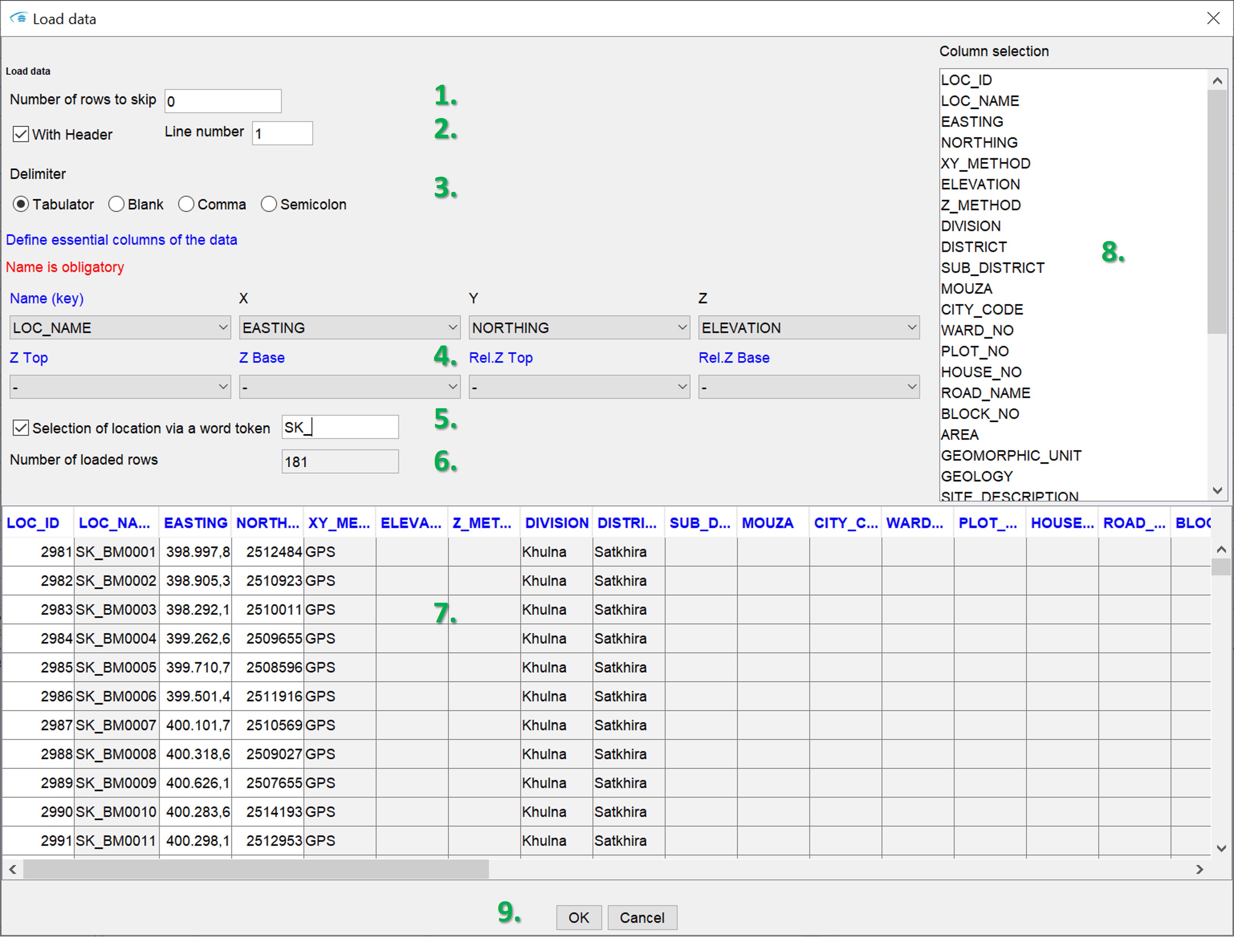
In the example, we have loaded any ASCII text table with the extension *.dat. Before the table is finally imported, you define the settings for the import via the user interface shown here:
- At Number of rows to skip you can set the number of rows to skip from the header of the file.
- With a tick at with header you tell the system that there is a title line. In the field behind it (line number), enter the line position of this title line in the file.
- Below this, use delimiter to specify the delimiter for your table.
- Now follows the section define essential columns of the data. This section is important if you want to create a data tree. Tell the system in which columns the georeferencing (spatial reference) of the data is stored. In the red font below, depending on the format of the table, you are given the hint which parameters should be occupied by columns that everything works well:
* Name: the planned primary key or location name or sample name. May vary for links.
* X: the column with the X-coordinate.
Y: the column with the Y-coordinate
Z: the column with the Z-coordinate (absolute, e.g. m NN), usually this is the drill approach height or the top of the ground, but it can also be other heights of point data.
Z Top: the column of the absolute height (Z) of the top of the depth interval to which parameters are to be linked.
Z Base: the column of the absolute height (Z) of the bottom edge of the depth interval to which parameters are to be linked.
* Rel. Z Top: the column of the relative height (Z) of the top of the depth interval to be linked to the parameter. This is the depth in relation to the top of the terrain.
* Rel. Z Base: the column of the relative height (Z) of the lower edge of the depth interval to which parameters are to be linked. This is the depth in relation to the top of the terrain. Note that loaded tables with relative heights should necessarily have a link to a table (or themselves) with information on the top of the terrain (Z) in order to obtain the correct spatial reference. - With Selection of location via a word token you can set a word part for location names. If you confirm this with ENTER, only those lines are imported that contain the corresponding word snippet in the location name (under name). If your drilling database is cleverly constructed, the location names are constructed with abbreviations for region memberships.
- Number of loaded rows shows the size of the final table to be imported.
- You will see a preview of the table as it is loaded. White columns show that the data stored here is numeric, grey columns correspond to the data type "Text/String".
- On the right side the column names are listed. You can select columns to be imported by making a selection. The columns not selected will be ignored. If you do not select anything, all columns will be imported.
- Press OK to import the table with your settings.
If the table has been loaded successfully, you will see it on the upper right side of the window with a new tab. The tab has the short name of the table. If you move the mouse over the title, you can see a tooltip that shows the number of rows and columns in the table.
All numerically loaded columns are shown in white and all text columns in grey. You can swap the columns with each other without changing the record itself. To do this, use the drag&drop function with the mouse on the header line. If you click with the mouse on the header of a column, the view of the table will sort itself according to the content of this column - always alternately ascending and descending. This only has a visual impact and does not change your invited record.
Note: You can only load one table at a time under the same path. If, for example, you have imported a part of the table and now want to load another part from the same source, you should save the part loaded first under a new path. To do this, use the save symbol at the bottom of the Table toolbar.
¶ Parser for layer descriptions
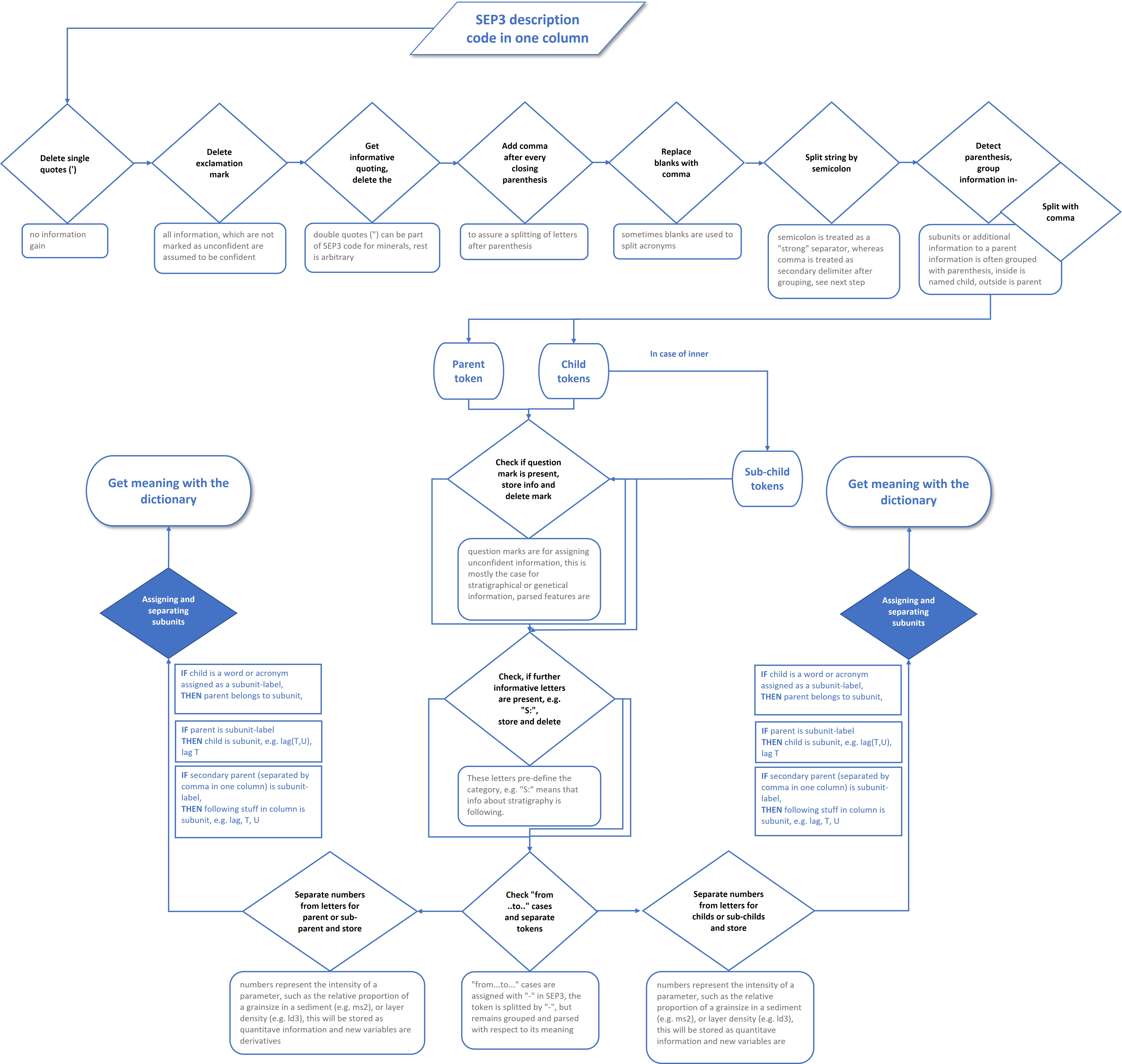
The parser for layer descriptions translates, structures and sorts certain sediment properties into a new table format that allows you to perform simplified analyses during your modelling. It was developed within the goCAM research project. The generated tables were used for a machine learning-supported labelling of sediments.
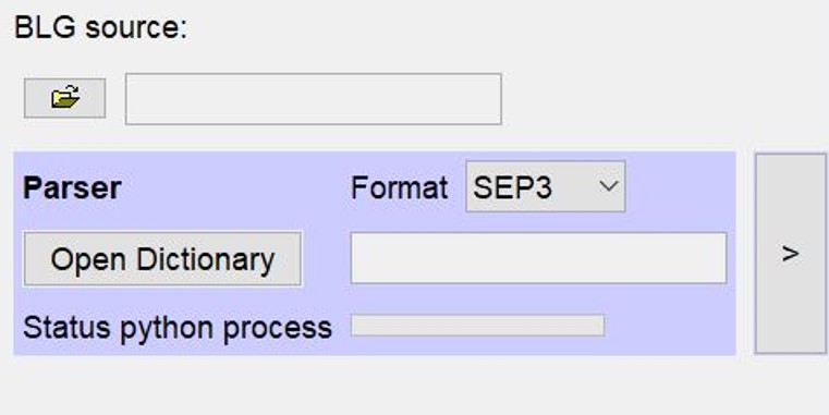
You can find this function in the blue-framed section on the upper left side of the Parameter Manager.
It can be set to translate shift descriptions with english syntax or with (SEP1/)SEP3 syntax under format.
**Try out whether the syntax of your layer descriptions is suitable for the parser. If not and you can share the syntax of your layer descriptions with us as an example, feel free to contact us. We would like to improve the parser in our further developments and extend it to multiple use cases. Furthermore, you should keep in mind that we have concentrated on the locker sediment area in our development. It is possible that you will not be able to use this functionality for your work with bedrock, or only with great caution.
In order to use the parser at all, Python must be installed. Read the notes on this in the introduction above.
You need a loaded *.blg-table. This table will be translated. You should follow the format template described in the linked article for the *.blg table. Lastly, you need to load a dictionary. We offer a template for this on request. Send us an email for this.
Start the parser with the big button on the right side in the field. If you have not defined a Python path in the programme settings, you will get an error message. Otherwise, the Info window opens. You will get information about the Python process. This will not be rendered until the process has completed. Note that with several tenthousands of entries of layer descriptions it may take a while until the translation is completed. You will receive a popup window with information about the completed process.
You will find the translated *.blg-file in the same folder of your input file. For storage, the same file name is stored with the addition _parsed. Another file with the same name and the addition _unknownWords is output. This is a table with two columns. In the first column, it lists the words that did not find a translation and in the second column, the name of the borehole where this word appeared. This gives the option of upgrading the dictionary or making corrections in the input file. You will see possible spelling mistakes in the layer descriptions that have prevented you from deriving information correctly. You can upgrade these in the Dictionary.
¶ Output of the parser and the dictionary
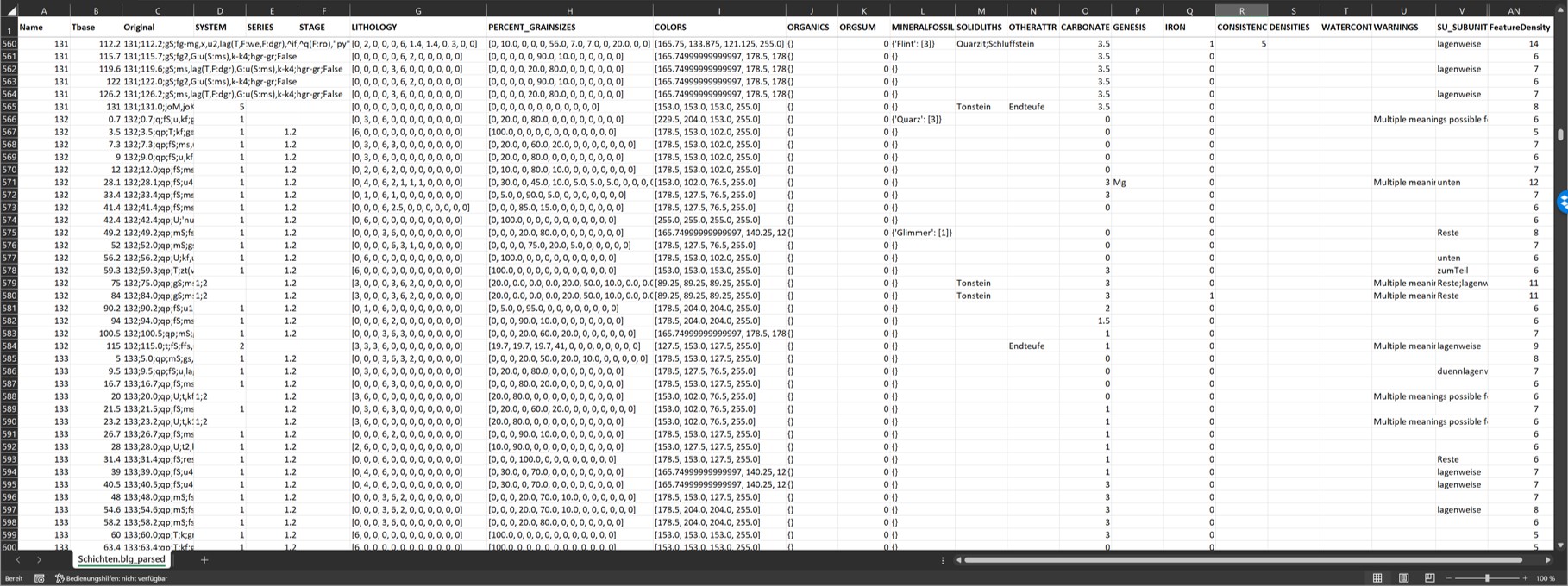
The output of the parser is a TAB-separated structured table in *.blg format. The first column contains the name of the borehole or the key of the layer description. The second column contains the depth in relation to the top of the terrain in metres. In the third column is the text of the layer description in the original, as it has been incorporated into the translation. If there is a "false" in the text, there were no identical layer descriptions in the file. A "true" indicates a duplicate. This is followed by columns that are discussed in the following sub-chapters.
Below this are the column WARNINGS and FeatureDensity. In WARNINGS all warnings of the parser are stored. Read this column and check the output for the hint mentioned there. The column FeatureDensity shows the number of entries in the layer description from which information could be derived. A high number indicates a detailed description, while a low number may be based on a rough layer description.
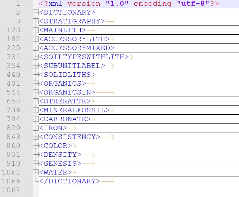
The Dictionary is a simplified XML file. It contains the mandatory categories in tags that would be regularly read from layer descriptions.
For each category there is a specific translation path with rules and a target format of the output.
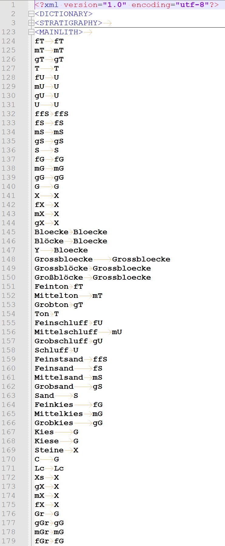
Within the tags of the Dictionary you will find simple two-column tables whose columns are TAB-separated. The first column contains the word or abbreviation you are looking for, which is to be assigned to the category and translated if necessary. The second column contains the translation, sometimes linked to specific rules. In many categories, the second column remains empty. Read the section below fopr more information.
Leave the tags of the categories in each Dictionary file in any case. The contents, i.e. the tables under the tags, may be edited or empty. The second column can be used to group terms and abbreviations with the same or similar meaning. This has great advantages in evaluation or for use in Machine Learning-supported labelling procedure (e.g. "lots of", "lots of" can be combined to "lots of", or "pieces of wood", "wood residues", "wood" to "wood").
Note:
You can give the *.blg-file a functional header with which you set further conditions to the parser.
If the names in the header of the columns in the *.blg header are all different from the tag names of the Dictionary, all categories of the Dictionary are tested for translation for each *.blg column.
A tag name in the header of a specific column means that for this column this category was explicitly assigned for translation. No other column would still be tested with this category.
If the tag name is entered with a prefixed * in the header, the column is tested for this category, but subsequent columns can be tested for this category.
You manage the assignment of several categories to one column with the entries of the names accompanied by a / separation.
The meanings of the Dictionary categories with their rules and output formats are listed below:
¶ STRATIGRAPHY
Rule and target format of translation:
The stratigraphy is treated in three parts in the parser, which means that for translation there are three columns in the output:
- SYSTEM: Ideally an ID (a representative integer) for the parent age, e.g. Quaternary, Tertiary, etc.
- SERIES: Ideally an ID (a representative integer) for the series of the age, e.g. Vistula, Drenthe, etc.
- STAGE: Ideally an ID or word for the stage of the series or a lithostratigraphic assignment, e.g. Coastal Holocene, Lauenburg Clay.
In the dictionary, the IDs for SYSTEM and SERIES must be combined by a dot, e.g. 1.2, 2.2, 2.3, etc.. STAGE is separated by a semicolon ;.
For example, the rule for a translation of the stratigraphy looks like this: qhKh TAB 1.1;Kuestenholozaen.
Use of the target format:
Translating the stratigraphic system and series into integers, or decimal numbers with one digit if necessary, enables you to communicate the stratigraphic assignments in their chronological order to computer-aided functions. This makes it easier to sort from young to old or vice versa. The tripartite division makes it possible to build up a hierarchy.
¶ MAINLITH and ACCESSORYLITH
The words and abbreviations used to describe the grain size group in the major (MAINLITH) and minor (ACCESSORYLITH) parts of the sediment are listed here. These categories are the most important part of the lithological description.
Rules:
The lithology is decisive for a large number of sediment parameters that can be derived from it, e.g. pore volume, hydraulic permeability, cohesiveness, relative swelling capacity and others. Therefore, special rules and target formats are provided for these categories (together with ACCESSORYMIXED and SOILTYPESWITHLITH).
The lithology can be entered in the first column as a word or abbreviation. For example, in the SEP3 syntax you will find "T" for "clay". You can enter the word "clay" directly. Non-conforming words or words with spelling mistakes occur in shift descriptions. If you have discovered this, you can enter them here and still have them translated correctly.
**The second column must be occupied. This time, the translation is actually based on the abbreviations from the SEP3 syntax and is done like this:
| Englisch | Translation Dictionary |
|---|---|
| Clay | T |
| Silt | U |
| Sand | S |
| Gravel | G |
| Stones | X |
| Blocks | Bloecke |
| Great blocks | Grossbloecke |
| _____________________________ | ________________________________ |
| finest (sands only) | ff |
| fine (sand & gravel only) | f |
| medium (sand & gravel only) | m |
| coarse (sand & gravel only) | g |
| _____________________________ | ________________________________ |
| clayey | T |
| silty | U |
| sandy | S |
| gravelly | G |
| stoney | X |
Note that in SEP3 syntax, the letters for the subordinate parts are written in lower case, but in this Dictionary you leave it in upper case. Whether something is a sub-genre part is determined by the rules of the parser and the words you assign in MAINLITH or ACCESSORYLITH.
"medium sand" would be entered with "mS", and "fine gravel" with "fG", just as "medium sandy" and "fine gravelly"
Internally, the lithology descriptions are also checked for intensities. For SEP1/SEP3, the integers are processed in the appendix of a lithology abbreviation. For English syntax, the position of the relevant keywords, which you can see below in the table as an example, is checked and assigned. For from-to cases are also checked.
| Englisch | Translation Dictionary |
|---|---|
| very strong (5) | 5 (35 - ~60 % -> 39.99 %) |
| strong (4) | 4 (25 - 35 % -> 30 %) |
| medium (3) | 3 (15 - 25 % -> 20 %) |
| slightly (2) | 2 (7.5 - 15 % -> 10 %) |
| very slightly (1) | 1 (2.5 - 7.5 % -> 5 %) |
A lithological description that reads, for example, "medium sand, silty, fine gravelly" would be translated as "mS(6), U(3), fG(3)". Internally, other processes take place with this information, which is explained in the follwing chapter.
Target format: The translated lithology is output in the output table as follows:
-
LITHOLOGY: here is a text in array form with the following order -> [clay, silt, finest fine sand, fine sand, medium sand, coarse sand, fine gravel, medium gravel, coarse gravel, stones, blocks, great blocks]. This list contains ordered integers for the intensity of occurrence in the sediment. The numbers correspond to the table above (1-5). Major parts of the sediment are given a 6. It may happen that only "sand" or "gravel" is given in the layer description without further subdivision into "fine, medium, coarse". If this is the case, assume that all three subcases are present in equal parts in the sediment. This is usually not the case, but a correct classification of subdivisions would be possible if this could be deduced from a genetic context of the sediment. Depending on the sediment genesis, there are differences. The parser cannot provide a "smarter" derivation. A warning is issued in the output column WARNINGS that there was a rough sediment description, so you can find these cases in post-processing and rework them if necessary.
-
PERCENT_GRAINSIZES: here is a text in array form with the following order -> [clay, silt, finest fine sand, fine sand, medium sand, coarse sand, fine gravel, medium gravel, coarse gravel, stones, blocks, great blocks]. The derived percentages of a grain size in the sediment are listed. The initial share of the grain size in the sediment is conservatively applied according to the table above. If the sum exceeds or falls below 100%, a correction is made. This ensures that the share of a grain size in the sediment with intensity 1 (=very weak) does not fall below the 5% mark and the declared main shares in total do not fall below the 60% mark. The result in this column can be compared with the results of a sieve grain analysis. The derivation is done with conservative approaches from the layer descriptions.
Important Note: Read the sections for ACCESSORYMIXED and SOILTYPESWITHLITH. Because these are categories that have an influence on the LITHOLOGY and PERCENT_GRAINSIZES columns.
Incidentally, if the information for lithology was accompanied by an abbreviation or word of a subunit, it will be treated separately. These details are listed in the columns SU_LITHOLOGY and SU_PERCENT_GRAINSIZES. "SU_" therefore stands for "Subunit". Rules for the subunits can be found in the workflow-chart of the parser.
Use of the target format: Especially the target format PERCENT_GRAINSIZES becomes usable in some other places in the Parameter Manager. With this you can have your derived sediment compositions displayed in a ternary diagram, classify sediment types manually or with clustering methods and output hypothetical distributions of hydraulic permeabilities. This column serves as a basis for calculating coarseness curves to display the lithology as a downhole curve in further plots.
¶ ACCESSORYMIXED und SOILTYPESWITHLITH
Here, the words and abbreviations of strata descriptions are listed that carry summary or indirect information on lithology. These are words such as: "loam", "loamy", "loess", "marl", "boulder sand", etc. In ACCESSORYMIXED it is the admixtures (e.g. loamy) and in SOILTYPESWITHLITH it is the descriptions of the main sediment (e.g. loam).
Rules:
For these keywords, the parser includes some conservative assumptions about the grain size fractions in the sediment, which we have taken from the literature (especially Quaternary and soil). The results are added to the output format for lithology, with preference given to MAINLITH and ACCESSORYLITH.
It often happens that these keywords are not accompanied by more detailed lithological descriptions. To avoid loss of information, you can consider this circumstance with the parser. The associated descriptions contain references to other sediment parameters, such as carbonate content (e.g. "loess", "marl"). These sediment properties are conservatively included in the set of rules.
If you do not want these keywords to be integrated, you can leave the two categories in the dictionary empty.
Note: You do not need to fill the second column for these categories if the term in the first column can be used for a translation, e.g. clay, marl. It is best to get our template of the Dictionary.
Target format: The translated lithology, as well as the carbonate content, is output in the output table as follows:
- LITHOLOGY: Read this section.
- PERCENT_GRAINSIZES: Read this section.
- CARBONATE: Read this section.
Important note: Be sure to look at the MAINLITH, ACCESSORYLITH and CARBONATE sections.
Incidentally, if the information for these categories was accompanied by an abbreviation or word of a subunit, they are treated separately. These entries are listed in the columns of the same name preceded by SU_.
Use of the target format: The target format PERCENT_GRAINSIZES becomes usable in several other places in the Parameter Manager. With this you can have your derived sediment compositions displayed in a ternary diagram, classify sediment types manually or with clustering methods and output hypothetical distributions of hydraulic permeabilities. This column serves as a basis for calculating coarseness curves to display the lithology as a downhole curve in further plots.
¶ SUBUNITLABEL
In this category list abbreviations and terms that indicate the occurrence of a subunit. The entries are important to avoid mixing lithological information on the main sediment with information on subunits.
Rules:
The rules for deriving a subunit are more complex, especially for the SEP1/SEP3 syntax. They can be taken from the workflow-chart.
The second column contains empty entries in this category. Point to the search for the term without translating it. The second column can be used to unify similar terms, e.g., "partienweise", "Partien von", "stellenweise" -> "partienweise". If you use this option, you will notice clear advantages later in the evaluation, as you can visualise and evaluate a variety of terms with the same or similar meaning together. This can have advantages for machine learning-supported labelling.
Note: Due to the diversity in the occurrence of possible layer descriptions, it is not possible to cover all cases for subunits per se with a set of translation rules, even if we have been able to include many cases. In principle, the more consistent the layer descriptions themselves already exist and are subordinated to certain rules, the cleaner the translation. A consistent strata database has advantages in any case. We may be able to include new rules if you discover one that has not yet been followed by the parser. Feel free to contact us.
Target format and benefits of target format:
All terms found as subunits and translated if necessary are listed in the output table with the column SU_SUBUNITLABEL. If there were several entries, they are separated by a ;.
All characteristics accompanied by a SUBUNITLABEL are listed in the output columns preceded by SU_. "SU_" therefore stands for "Subunit".
The contents of the SU_SUBUNITLABEL column can be visualised in a filtered manner. The spatial distribution and descriptive statistics can be examined with the manager parameter. The occurrence of subunits can reveal indications of sediment rearrangement in the modelling, for example. A clear visualisation will thus help you in the construction of your conceptual models.
¶ SOLIDLITHS
This category separately lists abbreviations or terms that describe solid rocks.
Rules:
Enter the search terms for solid rock descriptions in the first column. With the second column, you can combine similar or identical meanings of different descriptions into one target word.
Target format and usefulness of the target format:
The translation of this category is in the output table in the column SOLIDLITHS. For multiple entries in a layer, the results are listed separated by a ;.
All entries accompanied by a SUBUNITLABEL are listed in the output columns preceded by SU_.
The contents of the SOLIDLITHS column can be visualised in a filtered manner. If, for example, erratic blocks of a certain rock type are found in an ice-age deposit, they may provide valuable information on the transport routes or ice movement. The spatial distribution and descriptive statistics can be examined with the parameter manager. A clear visualisation will help you construct your conceptual models.
¶ ORGANICS and ORGANICSIN
This category lists separately abbreviations or terms describing organics (ORGANICS) or organic admixtures (ORGANICSIN).
Rules::
Enter the search terms for descriptions of organics or organic admixtures in the first column. With the second column, you can combine similar or identical meanings of different descriptions into one target word.
Target format:
The translation of this category is in the output table in the columns:
- ORGANICS: The output of organics and organic admixtures is a text in Python Dictionary format. The information is stapled in a curved way. Empty dictionaries look like this {}. The search term or the translated term is in single inverted commas '. Behind it you will find a colon :. It follows a list in array form with a square bracket and integers listed inside. Most of the time it is just one integer. These are the intensities of organic content found in the descriptions. Terms that correspond to the category ORGANICS are obligatorily given a 6, because it is assumed that this is the main component of the sediment. These are terms like "peat", "bog" or "mud". Use ORGANICSIN to assign the words and abbreviations for organic admixtures. If no intensity is found in the description, a 3 is automatically set for medium. If several intensities for the same translation term occur in this list, they come from different entries in the layer description.
- ORGSUM: This column lists the sum of the intensities or mentions found from the Python dictionary ORGANICS. It gives a relative measure of the occurrence and weight of descriptions of organics or organics content.
All specifications accompanied by a SUBUNITLABEL are listed in the output columns preceded by SU_. "SU_" therefore stands for "Subunit".
Use of the target format:
The contents of the ORGANICS column can be visualised in a filtered manner. The spatial distribution and descriptive statistics can be examined with the parameter manager. A clear visualisation will help you construct your conceptual models. The ORGSUM column gives you a relative impression of the organic content in a numerical format. This can be evaluated advantageously in certain cases and with good translation.
¶ OTHERATTR
In this category you can add all words and abbreviations of the sediment description that could not be assigned to any of the other categories.
Rules:
In the first column enter the search term that you want to find in the output table. The second column is for translation and is also a word or abbreviation, as desired. You can use the second column to combine words with similar or the same meaning into one target word. The second column may remain empty, in which case it is only searched for and assigned to the category, but not translated.
Target format:
You will find the result of the translation in the column OTHERATTR. If there are multiple entries for this from the layer description, the terms are separated with a ;.
All entries accompanied by a SUBUNITLABEL are listed in the output columns preceded by SU_.
Use of the target format:
The contents of the OTHERATTR column can be visualised in a filtered manner. The spatial distribution and descriptive statistics can be examined with the parameter manager. A quick, clear visualisation will help you in the construction of your conceptual models.
¶ MINERALFOSSIL
This category summarises the terms described for the mineral content and fossil content of sediment.
Rules:
In the first column enter the search term that you also want to find in the output table. The second column is for translation and is also a word or abbreviation, as desired. You can also use the second column to combine words with very similar or the same meaning into one target word. The second column may remain empty, in which case it is only searched and not translated.
Target format:
You will find the result of the translation in the column MINERALFOSSIL. The output of mineral and fossil content is a text in Python Dictionary format. The information is always stapled in a sweeping way. Empty dictionaries look like this {}. The search term or the translated term is in single inverted commas '. Behind it you will find a colon :. It follows a list in array form with a square bracket and integers listed inside. Most of the time it is just one integer. These are the intensities of mineral or fossil content found in the descriptions. If no intensity information was found in the description, a 3 for medium is automatically assigned.
All data accompanied by a SUBUNITLABEL are listed in the output columns preceded by SU_. "SU_" therefore stands for "Subunit".
Use of the target format:
The contents of the MINERALFOSSIL column can be visualised in a filtered manner. The spatial distribution and descriptive statistics can be examined with the parameter manager. A clear visualisation will help you in the construction of your conceptual models. If certain geological units show conspicuous occurrences of certain mineral or fossil contents, this will be reflected in the result of machine learning-supported labelling.
¶ CARBONATE
In this category enter words or abbreviations with references to the carbonate content of the sediment.
Rules:
In the first column, enter the abbreviation or word to be searched for or translated, as usual. Note that the abbreviation "k" in the SEP1/SEP3 syntax may be followed by an intensity number. This is considered in the parser, so you only have to enter the "k". You should list the "k" in the second column of the translation if you expect intensity information on the carbonate content. If you want to translate into "carbonate" with intensity = 3, enter "carbonate" in the second column.
For English translations, enter the word "calcareous".
For the meaning "calcareous", words must be translated with this keyword, i.e. "calcareous ". For the English translation, enter the words "non-calcareous " or "carbonate-free " in the second column.
Specifications such as "free of lime" or "non calcareous" will cause you difficulties in the translation because they are separated by a space and it may be possible that the parser does not recognise the context. You should catch such cases in your input file before the parser runs to get a correct translation.
Angaben wie "Kalk", "Kalkmudde" oder ähnliches funktionieren ebenfalls und erkennen das Sediment als deutlich kalkhaltig an. Wie sich das auswirkt lesen Sie in den Angaben zum Zielformat.
Target format:
The translation can be found in the CARBONATE column of the output table. This is a numerical entry. Search words for an existing carbonate content with intensities will receive the corresponding intensity number, as is the case with the LITHOLOGY. If no intensity information and/or the keywords "calcareous", "carbonate", "marl" or "loess" are present, a 3 is obligatorily set. Note that "marl" and "loess" can come from the category SOILTYPESWITHLITH or ACCESSORYMIXED ("marly"). Entries with "lime-free" or "non-calcareous"/"carbonate-free" will receive a 0 as numerical equivalent. All other entries in this category will receive a 5. If several entries occur in a layer description, a mean value is calculated. If there is no information on the carbonate content, there will be no entry in the corresponding line of the output, i.e. no number.
All data accompanied by a SUBUNITLABEL are listed in the output columns preceded by SU_.
Use of the target format:
The contents of the CARBONATE column can be visualised in a filtered manner. The spatial distribution and descriptive statistics can be examined with the parameter manager. A clear visualisation will help you construct your conceptual models.
¶ IRON
In this category you store search words and abbreviations that indicate an iron content in the sediment.
**Rules
In the first column enter the abbreviation or word to be searched for or translated. The second column must be entered and contains an integer. You can follow the intensity numbers used elsewhere in the parser. In our previous work, it was sufficient to use the 1 as a translation to merely indicate the presence, since an intensity could not really be derived.
Target format:
The translation can be found in the IRON column of the output table. This is a numerical entry and corresponds to the number you entered in the second column of the Dictionary. If no information on the iron content was available, a 0 is set here, in contrast to the carbonate content, since we have not yet encountered the information "iron-free".
All data accompanied by a SUBUNITLABEL are listed in the output columns preceded by SU_. "SU_" therefore stands for "Subunit".
Use of the target format:
The contents of the IRON column can be visualised in a filtered manner. The spatial distribution and descriptive statistics can be examined with the parameter manager. A clear visualisation will help you construct your conceptual models.
¶ CONSISTENCY and DENSITY
Here you translate information about the consistency or density of the sediment.
**Rules
In the first column enter the abbreviation or word to be searched for or translated. The second column must be entered and can contain an integer or a word. If words are entered, we assume an intensity specification in the layer description. The description should therefore be accompanied by such an intensity. If no intensity is found, it is automatically translated as 3. We recommend a sensible ordinal numbering scheme at this point, e.g. ascending for larger densities or firmer consistencies.
Target format:
The translation can be found in the columns CONSISTENCY and DENSITIES of the output table. This is usually a numerical entry and corresponds to the number you entered in the second column of the Dictionary. If from - to entries could be determined, mean values are output. Other multiple entries are listed separated by ;. These columns can contain numerical data as well as text data separated by semicolons.
All data accompanied by a SUBUNITLABEL will be listed in the output columns preceded by SU_.
Use of the target format:
The contents of the CONSISTENCY and DENSITY columns can be visualised in a filtered manner. The spatial distribution and descriptive statistics can be examined with the parameter manager. The information in layer descriptions that come from drilling archives is usually quite inaccurate. For an investigation of sediment consistencies and densities, we recommend consulting geotechnical field data.
¶ COLOR
Use COLORS to translate sediment colour information into RGBA equivalents.
Rules:
For the first column of the Dictionary use the abbreviations or words of the basic colours and colour attributes that are typically mentioned for sediment descriptions. The basic colours are, for example, "grey", "beige", "yellow", "green", "black" etc.. The colour attributes are additions that describe the expression of the colour, such as "dark", "light", "-light" etc.
In the second column, enter the RGBA values (red, green, blue, alpha) for the primary colours in the numerical scheme 0-255. List them comma (,)separated. Select colour values that are close to the sediment colour. A sediment described as "yellow" is not "squeaky yellow". For example, you can use the colour selection tool of the legend editor to pick out a realistic yellow sediment tone in RGB.
The sediment colours in the descriptions are compound words, such as "greyish yellow" or "yellowish grey". The composition is detected by the parser. The selection for the colour attributes "dark", "light" etc. is somewhat more complex. Here you have the possibility to enter an arithmetic operation yourself, for example to offset the influence of the attribute "dark" with the RGB values.
As a rule of thumb, higher RGB values or higher sums of RGB values correspond to brighter colours than lower values.
The arithmetic operations can be entered with simple operators, * for multiplication, + for addition and - for subtraction, followed by a factor. You can add the mark % to the factor if you want the factor to be a percentage of the present colour values between 0 and 255. You are welcome to take suggestions for such factors from our Dictionary template. We recommend to test out a few colour codes and their results to get to the most realistic colour translations for you from the descriptions.
Target format:
The translation of the output for sediment colours can be found in the output table under COLORS and, for subunits, in SU_COLORS. The format is a text in array form, i.e. the RGBA values are surrounded by a square bracket and within are listed, comma-separated, the values between 0 and 255. If no colour coding or description was present in the layer description, the RGBA coding for pure white "[255, 255, 255, 255]" is set at this point.
Use of the target format:
You can display the translated lithology in the ternary diagram in the parameter manager. If you select the COLORS column in this window as the colour attribute of the plot, the points in the ternary diagram will be displayed based on the RGBA values in the COLORS column. Ideally you will see the distribution of grain sizes together with the associated sediment colouration. This column is available for machine learning-supported labelling. Here we have had good experience with a dimensional reduction using a one-dimensional principal component analysis. This can be further used as a labelling feature or as a downhole curve together with the lithology curve.
¶ GENESIS
In this category, the described terms on sedimentary genesis are summarised.
Rules:
In the first column enter the search term that should be in the output table. The second column is for translation and is a word or abbreviation. You can use the second column to combine words with very similar or the same meaning into one target word. The second column may remain empty, in which case it is only searched and not translated.
Target format:
You will find the result of the translation in the GENESIS column. If multiple entries are available, they are listed ;-separated.
All specifications accompanied by a SUBUNITLABLE will be listed in the output columns preceded by SU_.
Use of the target format:
The contents of the GENESIS column can be visualised in a filtered manner. The spatial distribution and descriptive statistics can be examined with the parameter manager. A clear visualisation will help you in the construction of your conceptual models.
¶ WATER
In this category, notes or abbreviations concerning the water content are entered.
**Rules
In the first column, enter the search term that should be in the output table. The second column is for translation and is also a word or abbreviation. The second column may remain empty, in which case the search is carried out. Decisive for the parameter WATER, is the fact whether something is water-bearing or not and how strongly. In the SEP1/SEP3 syntax, an intensity number can be placed after the abbreviation for water-bearing, similar to what you have already read above for the lithology. This is primarily used for translation, because either something is water-bearing or it is not.
Descriptions whose meaning is "dry" should be translated as "arid" or "dry", which then corresponds to the intensity number 0.
Target format:
You will find the result of the translation in the column WATERCONTENT. The intensity numbers are entered that were read out in the shift descriptions for the keywords or abbreviations. If no intensities were given, a 3 is obligatorily set. In the case of "dry", 0 is entered. If from-to cases are found, an average value of the intensity is formed. If no information on the water content was available, no number is entered.
All data accompanied by a SUBUNITLABEL are listed in the output columns preceded by SU_.
Use of the target format:
The contents of the WATERCONTENT column can be visualised in a filtered manner. The spatial distribution and descriptive statistics can be examined with the Manager parameter. Possibly, correlations to other described sediment characteristics and the water or moisture content of the sediment can be derived.
¶ Workflow chart of the parser
The workflow chart should help you to understand the basic rules for decomposition and interpretation of the layer descriptions. Since the SEP1/SEP3 decomposition is the most complex, most steps are assigned to this syntax.
¶ Working with tables
You can see the invited tables in the upper right section of the Parameter Manager. The tables are sorted into tabs. If you click on the tab of your target table, it comes to the foreground and thus becomes active for analysis and editing options.
Tip: Note the scroll bars on the right and below. With some window sizes, you may have to enlarge the section for the tables so that you can work with the scroll bars of the tables.
You have a toolbar below the tables that allows you to link, edit, analyse, save, and remove tables.
Note: The tools integrated here are for quick editing in typical processes of conceptual geological modelling. The Parameter Manager cannot be compared to a spreadsheet tool or a data management system in terms of scope.
If you want to sort a table for a specific parameter, click on the header of the relevant column. If you click again, the sorting will be inverted. You can adjust the column size if necessary. Go with the mouse into the header line and move the right margin there. With Drag&Drop into the header of a row, you can swap entire columns. Change the view of the table, but not the data set itself.
There are white and grey rendered columns in your table. The data in the white columns was internally recognised as a numerical data series, the grey columns correspond to text data (data type: string). If a data series was recognised as data type:Integer, i.e. integers, -99999 is inserted as NoData value if in the row the entry was empty.
¶ Toolbar for tables

-
 Link tables: Here you set table links. Load all the tables you need. It is advantageous if you have defined the columns for georeferencing before linking tables (read here) or have worked with point 2. A window opens which is initially empty, as there are no links at the beginning. With Add link you add a small field with further buttons.
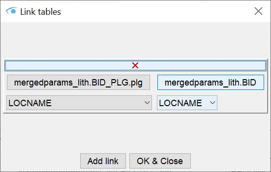
Each field represents a link. With the red X at the top of this field you can delete the link. Otherwise you will see the buttons Choose table 1 and Choose table 2. Select the two tables you want to link. As soon as you have selected tables, the dropdown lists below them are filled with the column titles. Here you now select the column for each table where the key for the link is contained. When you have finished with all the tables, press OK & Close and your links will be saved. You can create links up to a theoretical depth of 10 tables. Depth means the number of tables that can be linked from the table with the target parameter to the table with the georeferencing. There is a maximum of three link levels. In the article Integrating Parameters we have created a practical example.
-
 Allocate columns anew:
  With this tool you open a small window with which you can transfer the table contents with georeferencing to the system. If you have forgotten this step when loading a table, you can now do so with this tool.
 -
 Convert column(s) to numeric: If you use this button, a window appears with a list of those columns that currently contain data saved as text. By selecting the relevant columns, you can convert them into a numerical data series. This is useful if you have a data series that is actually predominantly a numerical series, but due to a spelling error in one row, for example, the entire data series was interpreted as text. Text that cannot be converted into numbers is translated as a NoData value. Note that there is no back for this. If you do not like the result, you will have to remove the table and reload it.
 -
 Convert column(s) to text: This tool is the reverse counterpart to 3. Use it to convert a data series integrated as a numerical series in the system into a text data series. This can be useful, for example, if you have loaded a series with label IDs and want to examine them with quantitative descriptive statistics rather than numerical statistics. If you do not want to have the column with the drilling location names integrated as numerical values, because this would be disturbing for a clean table linkage, a text conversion might make sense.
 -
 Editing column: This tool enables a column for editing. Unlike in relevant table editing programmes, you cannot write directly into the data series in the Parameter Manager. We have restricted this in favour of the links and the data tree. If you want to change values, you must select a column from the dialogue that appears when you use the button. The active column is highlighted in yellow and is active for editing. Click in the appropriate cell that you want to change. Note that you can insert only numbers in numerical data series (white columns). With STRG-Z you can return to the original value.
 -
 Delete chosen column(s): Here you can select from a list of columns in the active table which ones you want to delete. Columns that have been passed to the system as relevant for georeferencing cannot be deleted and therefore do not appear in the list.
 -
 Split text column:
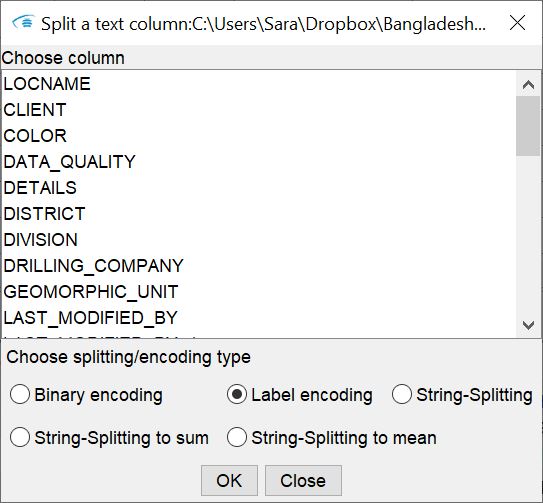
Here you can select columns whichs textual content is to be converted, for example in preparation for machine learning-supported labelling. The conversion and splitting options are:- Binary encoding: New columns are inserted into the table for all entries or keywords of the same type (from the selected column). These columns are given a compound title: "Title of selected column_" + "BIN_" + "Entry/keyword ". In rows that contain the corresponding keyword assigned to the column, a 1 is set. If the keyword is not included but no NoData value is set, you will see a 0, or a -99999, our NoData value for integer data series. If the text columns to split come from the parser for layer descriptions, this type of conversion cannot be done with text in array format. If the selected column is in Dictionary format, the binary encoding is done on the textual portions of the Dictionary entry. Thus, an empty Dictionary entry ({}) corresponds to a NoData value, while an entry as "{'Wood':[3], 'Roots':[3]} is converted into two columns - one titled "Wood" and one titled "Roots", which contain a 1 in the corresponding line. In the same way, the splitting and conversion is done for text contents listed in the selected column separated by ;. The binary encoding can bring advantages in visual analysis as well as in certain machine learning-based labelling processes. This method can be used to prepare data for categorical indicator kriging.
- Label Encoding: A column is added to the table with the following title scheme: "Title of selected column_" + "LABEL ". Each entry of the same type found in the selected column is given an integer equivalent. It is a translation of words into an integer coding. No splitting takes place here, as with the Binary Encoding above - it is a simple conversion. Label encoding can also be used in machine learning-based procedures or as preparation for indicator kriging.
- String Splitting: String splitting involves splitting a selected column of text into multiple columns and depending on the text format. Text in array form, as created by using the parser for layer descriptions, is separated into the individual elements of the array. Columns with the title scheme are created: "Title of selected column" + "_SPLIT" + "_ID of array position ". If you have a text in the translated-Dictionary format, a column is created for all entries found, as with the Binary Encoding: "Title of selected column" + "_SPLIT" + "_keyword ". The number from the dictionary array part is in the corresponding columns. If necessary, read the sections on Parser for layer descriptions to better understand the meaning of the formats. If you have a text column with a ;-separated word list, then for the maximum number of words found in these lists, columns are created that have the following title scheme: "Title of the selected column" + "_SPLIT" + "_ID of the newly created column ". I.e. in this case it is only a pure string splitting based on the ;. The string-splitting can be useful especially for a subsequent simplified representation of the contents from the translation of the layer description.
- String-Splitting to sum and String-Splitting to mean: These conversions split text columns in the array format of the parser. However, they are then merged into one column with the sum or mean of the array entries. The titles of the columns are composed like this: "Title of selected column" + "_SPLITMEAN/_SPLITSUM ".
-
 Standardize selected column: Here you select a column with numerical contents via the dialogue. The data is transferred with a z-score conversion to a new same-name column with the addition _standardised.
 -
 Scale column with minmax: Here you select a column with numerical contents via the dialogue. The data is then transferred with a min-max scaling to a new same-name column with the addition _minmaxScale.
 -
 Log-ratio Transformation:
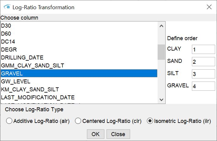
Here you select several numerical columns via the dialogue that opens, each of which is part of an otherwise self-contained sum. A good example are the columns of a sieve grain analysis, whose content represents the respective percentage share of a grain size in the sediment. The sum of each line from these columns is always 100%. Use this function carefully - because the plausibility of your column selection is not checked. You can choose between three different methods:- Additive Log-Ratio (alr) -> here you must additionally define the order of the columns for the transformation on the right-hand side. To do this, enter an integer for the position of the column in the field next to its title. For the definition of the base of this function, let the dialogue guide you through it after you pressed OK.
- Centered Log-Ratio (clr) -> this transformation is performed as soon as you confirm with OK.
- Isometric Log-Ratio (ilr) -> here you specify the order of the columns for the transformation on the right-hand side. To do this, enter an integer for the position of the column in the field next to its title.
Depending on your selection, you will see the results or the transformed data in the added columns with the additions alr, clr or ilr. Please note that with the additive as well as with the isometric log-ratio transformation basically a dimension reduction by 1 takes place. In the additive transformation, the column taken as the base is 0 everywhere after the transformation. In the isometric transformation, it is the column at the bottom of the hierarchy that contains 0 everywhere after the transformation. We have nevertheless added these columns for the sake of completeness and for better traceability.
-
 Show statistics to the column:
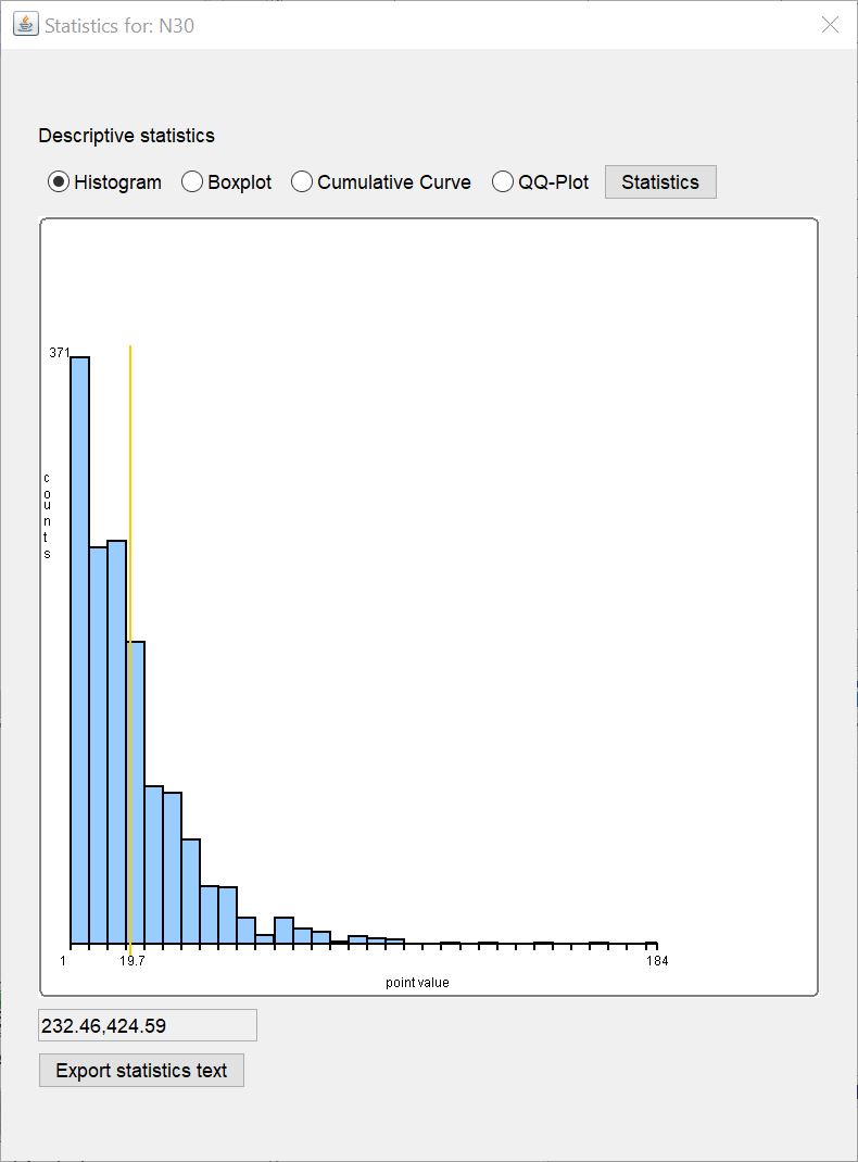
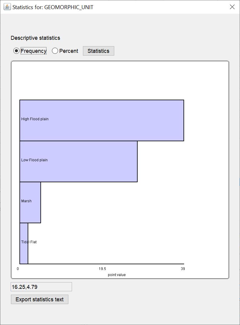 This button opens a list of all columns in the active table. Numerical and text data series can be checked for descriptive statistics. Select the column you want to examine and press OK. The familiar window for descriptive statistics opens. Details on the displays can be found in this article.
 -
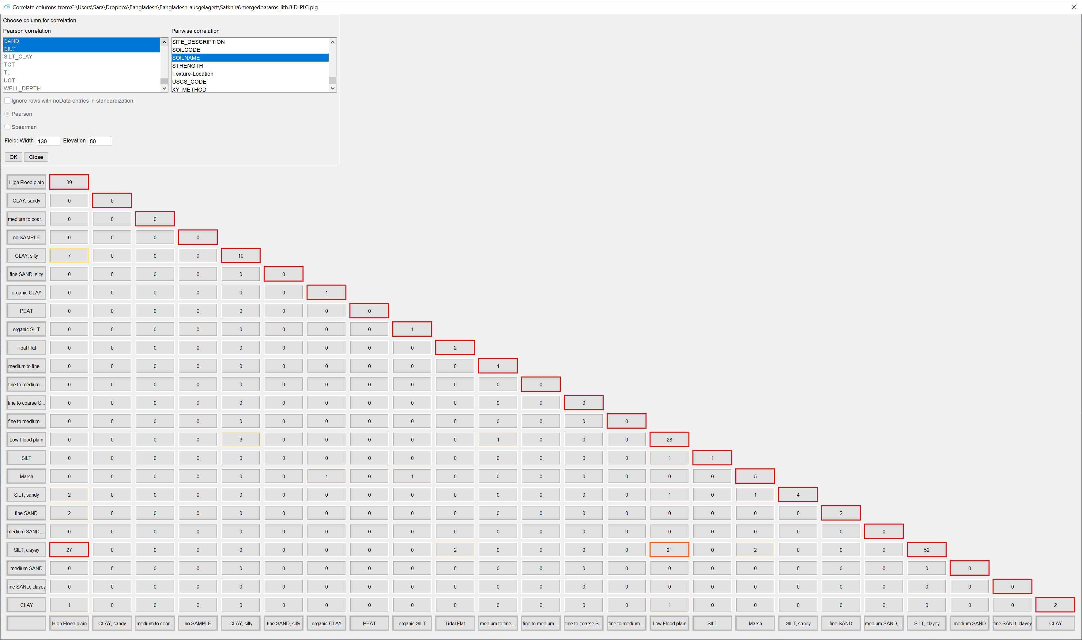
 Correlate columns: This opens a window with which you can check the correlation between parameters from the active table. Two lists are at the top. Numeric columns are listed on the left and text columns on the right. If you click with the mouse in the left or right list, you can select the target parameters using the STRG key. For the left list, the options Pearson and Spearman as well as Ignore rows with noData values in standardization become active for selection.
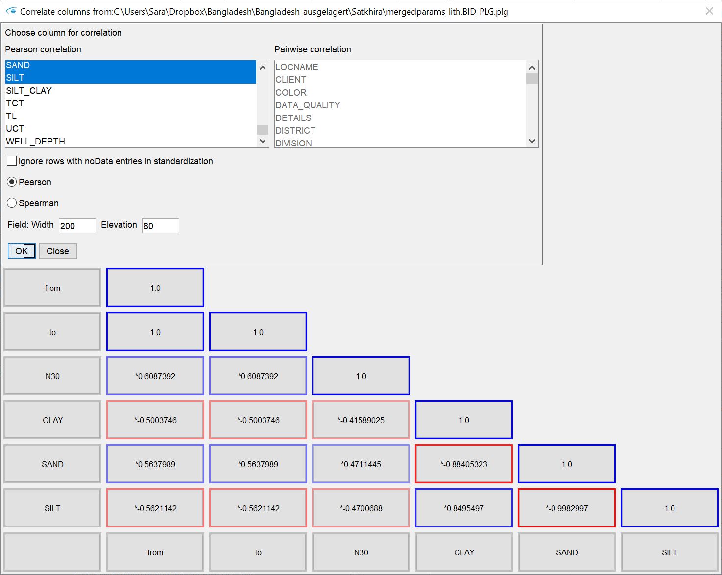
For Pearson and Spearman, select the output of the Pearson or Spearman correlation coefficient. For Ignore rows with noData values in standardization, you specify whether the z-score standardisation accompanied by the calculation is to be carried out with all values of a column or those in which all parameters whose correlation is to be checked also contain data, i.e. no NoData values occur.
If you select columns from the right list, the keywords from the text columns are checked for occurrence in pairs and inserted into a matrix. If you have selected text columns that contain ;-separated word lists or texts in Dictionary format that originate from the parser for layer descriptions, an internal string-splitting is used to correctly check the keywords for pairwise occurrences. For such columns, you should select only one of these columns for analysis.
You can select either numerical correlation or pairwise occurrence of text contents. Confirm with "OK". In both cases, if several parameters are present or selected, a diagonally divided matrix is created, which is made up of fields. The two dialogue input fields Field: Width/Elevation determine the size of the fields that contain the information of the output. You can change the field size at any time by entering a new value in the text fields provided and then pressing ENTER.
The outer lower and right margins always contain the names of the parameter pair or the word pair for whose correlation value/occurrence the field is to be found in the corresponding row and column. The upper diagonal margin always contains a 1 in the case of numerical data, because the parameter is of course perfectly positively correlated with itself, which corresponds to a correlation coefficient of 1. In pairwise observation, the sum of all pairwise occurrences of this word is written here. In the numerical case, you can read the selected correlation coefficients in the fields within. In the text case, you will find the number of pairwise occurrences of the respective word pair.
In the numerical case, correlation coefficients that indicate a positive correlation are marked in blue. The colour saturation indicates the strength of the correlation. Negative correlations are marked red accordingly. An "*" in front of the number indicates a positive significance test (p-value, two-sided t-test). When analysing words in pairs, the number of pairs with a high weight will be marked more red so that you can find them quickly.
If you hover your mouse over one of the fields in the matrix, you will get more information in a tooltip. In the numerical case, you will see the specific p-value that was calculated in addition to the correlation coefficient. In the paired word case, you will see the percentage share of the count in the sum of the paired occurrences of both values. The first percentage is always related to the column and the second percentage is always related to the row.
If more than 200 word pairs occur when you select your text columns for pairwise consideration, you will receive a warning. This is because the matrix cannot display more than 200 pairs. This would be impractical for a user to analyse anyway.
-
 Save table: Here you save the active table in a new file. The selection of the extension is only for your assistance in table administration. When saving, no format changes are made due to an extension. If the saving was successful, you will find the new table name in the header of the table tab. If you have linked tables or created a data tree, check the links again and create a new data tree.
 -
 Delete table: Remove a table from the parameter manager. If you have linked tables or created a data tree, check the links again and create a new data tree.
Note: If you have created links and data trees and are using editing and conversion functions in the tables, check the links again and create a new data tree.
¶ Parameter Funktionen
The parameter functions can be found in the Parameter Manager window on the bottom right-hand side as buttons. The user interface of the selected function appears in the lower left window. They are divided into four topics:
¶ DataTree
These are the general functions related to the creation and use of the data tree.
¶ DataTree
![]() With this button you create a data tree. It is the only function without a user interface. Since the data tree is very essential for many other functions for parameters, you should read the linked article about it. The icon has a blue border if a data tree is present in the system and no changes are present or suspected. In the latter case, the border is red.
With this button you create a data tree. It is the only function without a user interface. Since the data tree is very essential for many other functions for parameters, you should read the linked article about it. The icon has a blue border if a data tree is present in the system and no changes are present or suspected. In the latter case, the border is red.
¶ Filter & statistics
![]() This opens the user interface of the filter function for parameters. The filter is integrated with the same structure for raster and voxel objects. Read more about it here.
This opens the user interface of the filter function for parameters. The filter is integrated with the same structure for raster and voxel objects. Read more about it here.
¶ Project View
![]() With this function you open the user interface for creating a LocView object. Read the linked article to get more information. Here you define the legends for the colour representation of the loaded parameters, which affects the representations in the graphs of the Parameter Manager. We summarised the colour management with the article linked above.
With this function you open the user interface for creating a LocView object. Read the linked article to get more information. Here you define the legends for the colour representation of the loaded parameters, which affects the representations in the graphs of the Parameter Manager. We summarised the colour management with the article linked above.
¶ Lithological Analysis
Here you can carry out further lithological analysis and have hydraulic permeabilities estimated.
¶ Soil type module
![]() This function is only available if a data tree exists in the system.
This function is only available if a data tree exists in the system.
In the user interface you will see two sections left and right.
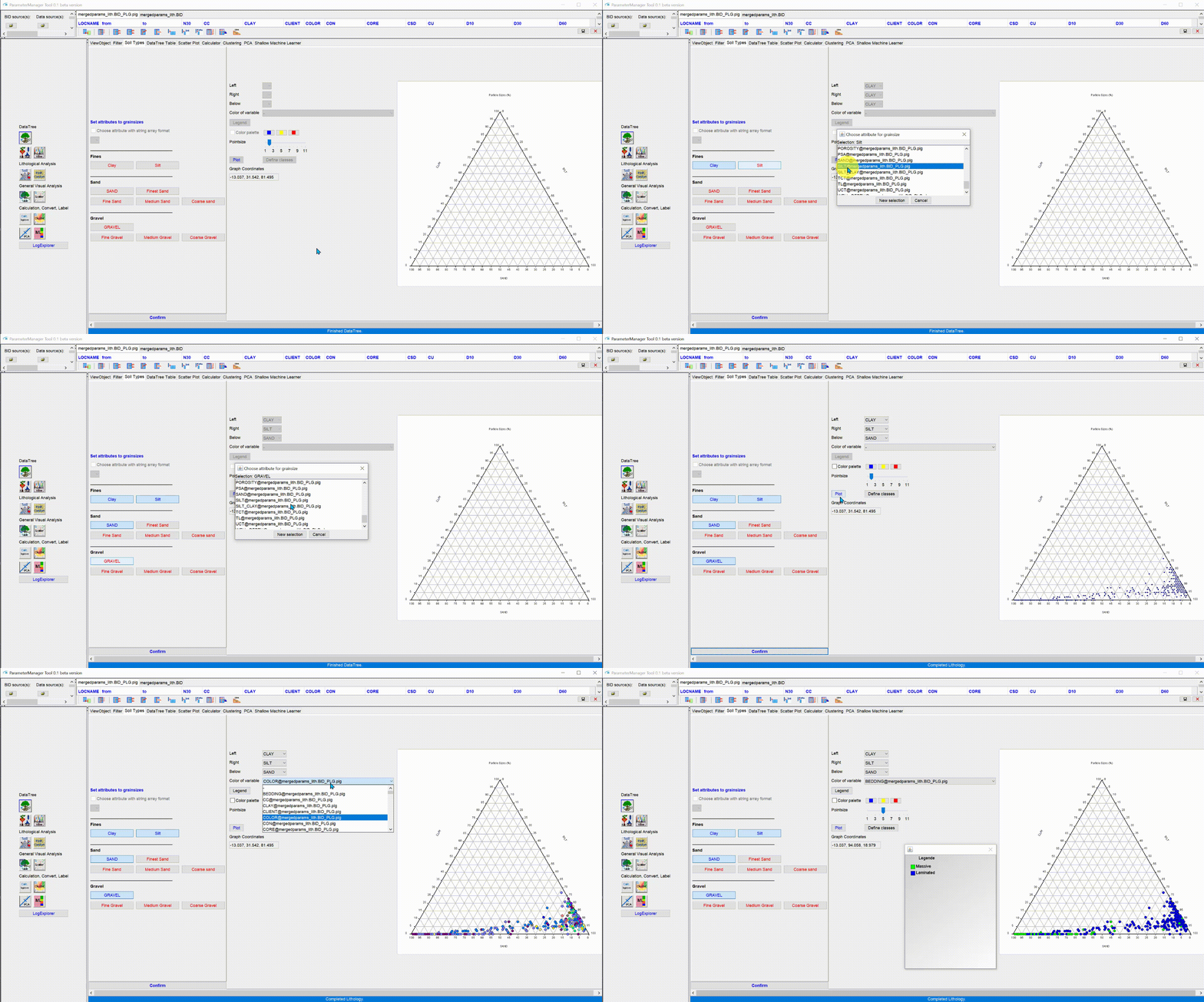
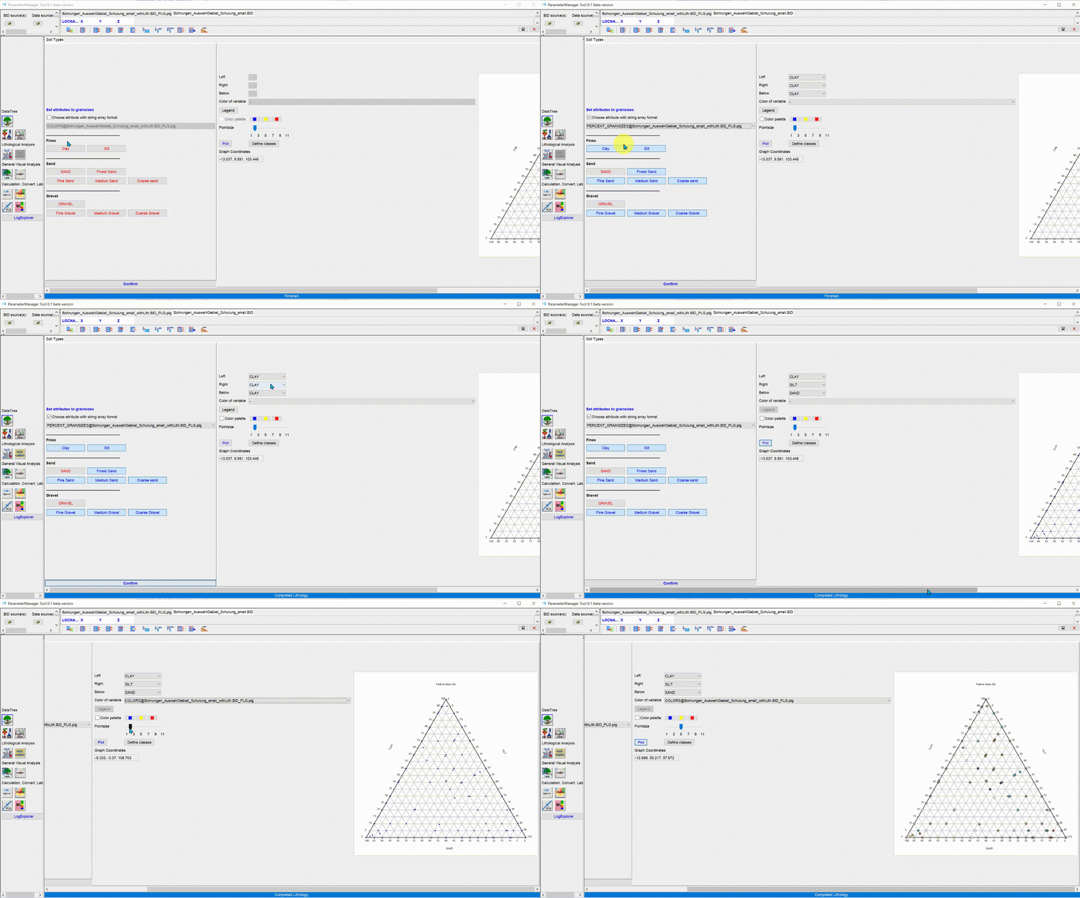
Left assign parameters to the system that contain lithological information or the percentages of grain sizes in the sediment. For correct processing, the sum of the selected parameters must add up to 100%.
If you have worked with the parser for stratified descriptions and there are no sieve grain analyses at all, you can check the Choose attribute with string array format box. The dropdown list below will become active and show those parameters that contain texts in array format. As soon as you select the parameter name PERCENT_GRAINSIZES, the buttons under Fines, Sand and Gravel will turn blue, corresponding to the assignment by the parser. If necessary, read the section on lithology. Buttons that remain red have not been given a correspondence. You can create your own text-array-formats externally and assign the respective positions in the array using the buttons under Fines, Sand and Gravel. To do this, press the button whose grain size is to be set and select the number for the position in the array from the list. You always confirm with new selection. If you press New selection but there is no active selection, the button is set to red again to shows you that the assignment has been deleted.
If you have parameters in the data tree that originate from one or more sieve grain analysis(s), you can assign the corresponding parameters from a list to the corresponding grain sizes using the buttons under Fines, Sand and Gravel. Multiple selections in the selection dialogues are possible and are best selected with a click and STRG.
If you Confirm, the lithology information is transferred to the system. In the process, SoilType objects are created internally at the corresponding coordinates, which contain the lithological information in the data tree. The SoilType object carries out various steps:
- It checks the incoming lithological information for completeness, i.e. whether the sum of the grain size fractions adds up to 100.
- It assigns intensity numbers for the grain size fractions according to the model of the parser for layer descriptions. On this basis, initially, and as long as you have not made any Sediment Classification, a text is generated which returns a sorted SEP3 description in German language setting of the SubsurfaceViewer and a sorted English description of the lithology in English language setting. So you can either generate a lithological description from a sieve grain analysis or bring existing lithological descriptions into a uniform form this way. You will find this initial description in the parameter "LITH_CLASS". If you make other sediment classifications, the initially generated description is overwritten with the new classification. You can restore the initial status if you reload the data tree and the lithology. If you want to keep these descriptions and still make a sediment classification afterwards, you ahould export a table [extracted from the data tree](#table-extraction). Reload the extracted table and create SoilType objects with which you can classify. If you have any questions about this, feel free to contact us.
- It passes the correct data to a ternary plot with defined axes.
- It calculates downhole curves for the coarseness (LITH_COARSENESS), the tendency of the minor constituents (LITH_TREND-> finer or coarser than the main constituent) and the degree of mixing (LITH_MIX) of the sediment. You can read how these curves are calculated, for example, in the publication of the goCAM project.
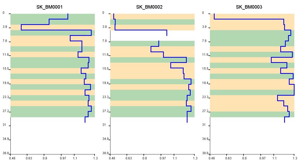

In the example you can see the coarseness curve (LITH_COARSENESS) at different drilling locations. In the section they are combined with other parameter representations in the cross-section view of the standard user interface. The lithology is shown towards the right. The somewhat paler and unfilled curves to the left correspond to the results of pile core probing.
To understand this, it is best to look at the examples in LocView Object and in LogExplorer. In the article Integrate Parameters you will find instructions on how to use these curves. - It saves lithological classifications you have made either with the HCE-Module or with the manual classification in the ternary diagram. You can find it under the parameter name LITH_CLASS.
- It passes the most important lithological information to the HCE-module for calculating hydraulic permeabilities from theoretical or measured grain size distributions of the sediment.
**On the right you see an initially empty ternary diagram and on the left of the graph some setting options. With the Dropdown lists Left, Right and Below you define the grain size group on the axes of the ternary diagram. The diagram is oriented clockwise, which you can see from the axis labels. Under Color of variable, select a parameter from the data tree that is responsible for colouring the points in the ternary diagram. For colouring, the parameter must have a frozen coordinate that corresponds to the SoilType object that is to be displayed as a point in the ternary diagram. If you have loaded a table of the parser, select the COLORS column that the points are displayed with the resulting RGB colours of the parser, which ideally corresponds to the sediment colouring. You can also create an externally generated RGBA data series for the lithological coordinates. If you select another parameter for colouring, the associated points of the lithology will be displayed with the internally predefined or the manually defined legend in the Project View window. The button Legend opens a window with the representation of this legend. With Color palette and the following three colour buttons, you can create a three-level colour palette specially tailored for this plot and display it here. With Pointsize you can adjust the size of the points in the ternary diagram. Press Plot to see the lithology in the ternary diagram. In the text field Graph coordinates, the coordinates of your mouse position update when you move it in the diagram. The same order applies here as was defined above with the Dropdown lists of the axes.
The button Define classes opens a new dialogue with which you can manually classify lithologies. Details on this can be found in this article.
¶ HCE module
![]() HCE stands for Hydrological Conductivity Estimation. It derives possible distributions of hydraulic permeabilities from created SoilType objects with class assignment.
HCE stands for Hydrological Conductivity Estimation. It derives possible distributions of hydraulic permeabilities from created SoilType objects with class assignment.
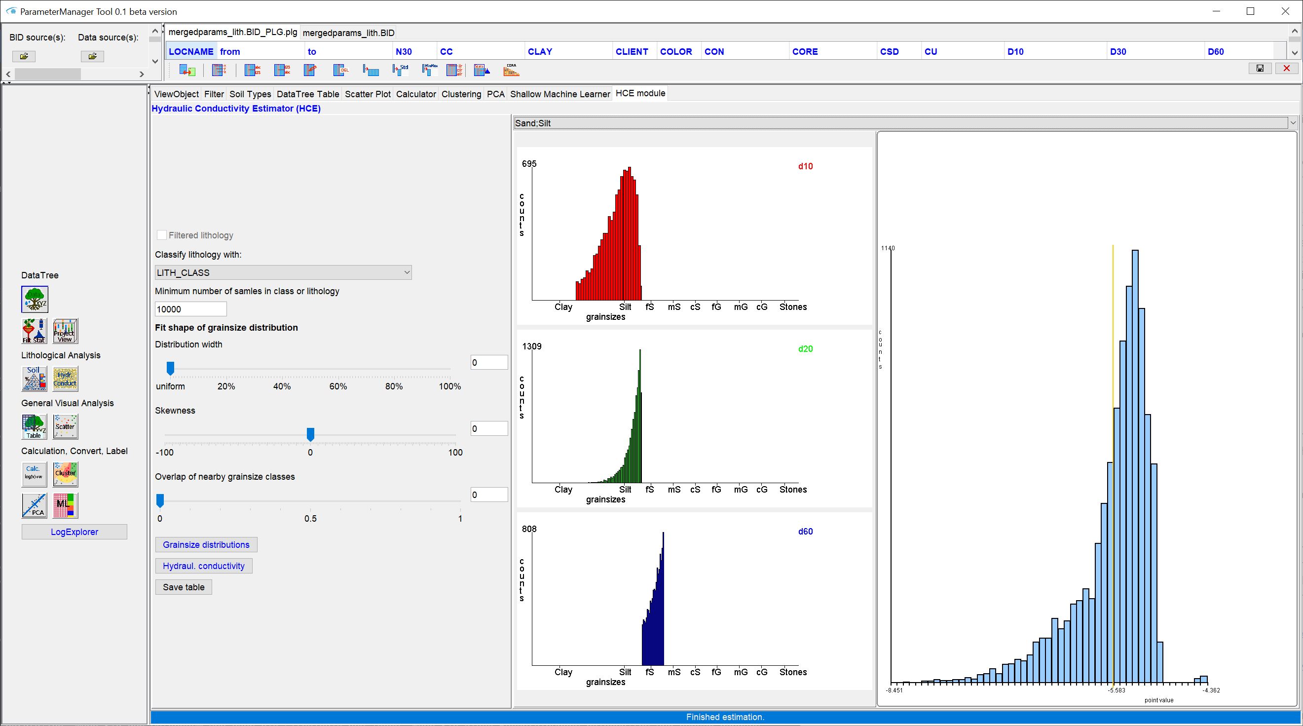
The idea originates from the goCAM research project and was somewhat simplified for implementation in SubsurfaceViewer in favour of manageability and performance. In short, possible distributions of concrete grain sizes (mm) for the percentiles d10, d20 and d60 are sampled from data of grain size fractions (percentage for clay, silt, sand, etc.) by means of a random generator and adjustable conditions.
**A sample corresponds to a vector with one grain diameter value each for d10, d20 and d60 with the conditions of a grain sum curve, i.e. d10<d20<d60.
The assignment of grain sizes in mm to the grain size groups clay, silt, fine sand, medium sand, etc. is based on DIN 4022.
From these sampled theoretical grain size percentiles, the hydraulic permeabilities are then calculated as kf-value in m/s for each "artificially" generated sample using relevant formulae. The choice of formulas used are derived from the program manual of UK32, prepared by the authors: Dr. P. Szymczak, G.E.O.S. Freiberg Ingenieurgesellschaft mbH, M. Wassiliew, A. Behnke, HGC Hydro-Geo-Consult GmbH, Freiberg; status: version 1.2, August 2012, and published by the Saxon State Office for the Environment, Agriculture and Geology (Wittmann was neglected for lack of reliable porosity data).
Note: The HCE module can be further developed. We would be happy to discuss this with you if you have any suggestions for improvement or questions. Our focus was on evaluating a large amount of layer information on a regional scale for this parameter quickly and easily. That is why we chose to sample by percentiles instead of simulating hypothetical grain sum curves in the whole.
The user interface is divided into two parts. On the left you see options for estimation and on the right are shown graphs of the results.
The field Filtered lithology, which is inactive, is for information. If the check mark is set, you have previously applied a Filter to the Data tree.
The basic procedure for estimating hydraulic permeabilities is like this:
-
Determine whether there should be a lithological classification. With Classify lithology with you select an attribute that is linked to the lithology, i.e. is located at the same frozen coordinates in the data tree. This can be, the result of clustering over the grain size groups. If you select LITH_CLASS, the Sediment Classification currently active in the data tree will be used. If you select "-", the lithology dataset, filtered in advance if necessary, will be considered as a whole. Please note that if you select a new attribute, you will overwrite a manual sediment classification that was saved in LITH_CLASS. It is therefore best to save your manual classifications that you can reset them if necessary. How to do this, is described in the article on classification. You will receive a warning when a classification exists.
-
Under Minimum number of samples in class or lithology you define the minimum number of samples (SoilType objects) that should be present in a group/class. Initially, a number of 100 is suggested here. The proposal is chosen cautiously. This selection makes sense, if you group via a layer ID, i.e. basically a layer description also forms a group in each case. For a random sampling of grouped lithologies, and thus several layer descriptions or sieve grain samples together, it is usually better to use several thousand to hundred thousand samples. Try it out and choose the best ratio in terms of performance and result. If a lithological class contains fewer samples, the minimum number you have specified, the data set is duplicated in its entirety until the minimum number has been exceeded.
-
Decide what a distribution of possible grain sizes within a hydraulically effective grain size group (clay, silt, fine sand, medium sand, etc.) should look like. Based on the formulas used, we understand hydraulically effective to be the percentiles for the grain diameters d10, d20 and d60. If you leave everything in the default settings, a random generator will sample all associated grain sizes of the corresponding grain size group with the same probability for these percentiles. These are uniform distributions. If you move the slider Distribution width away from uniform, a normal distribution is sampled. The percentages of the slider refers to an assumption for the width of the distribution. At 100%-opening, the standard deviation of the normal distribution is half of the assumed range between the minimum and maximum possible grain size. If you move the slider Overlap of nearby grainsize classes away from 0, you set the minimum and maximum limits for grainsizes of a group to a percentage overlap with the groups on the left and right. An overlap greater than 0 automatically expands the width of the distribution that was set above proportionally to the range between minimum and maximum. An overlap value of 1 means that all grain sizes from the neighbouring grain size groups have a probability of being sampled according to the distribution. With the slider under Skewness you give the system a skewness of the distribution. As soon as you click on Grainsize Distribution, you will get a graph of the result in the form of histograms on the right. Please note that the graphs on the right are logarithmic and therefore a normal distribution does not appear in the usual form.
-
Now you have to press the button Hydraul. conductivity to complete the calculation. You will get a protocol of this in the Info-window and the histogram of the logarithmised kf-values from the calculation will be displayed on the right side.
-
If you want to archive the results in table form or use them further, export a file with Save table. The most important parameters of the calculated kf-value distribution in m/s (mean value, median, IQR limits, minimum and maximum) are output in the corresponding columns with coordinates and depths.
Note: You can reload the exported table with the kf-values into the Parameter Manager and increase your data tree. Then you have spatial filters and visualisations available for the kf-values, which might be helpful for the calibration of groundwater models.
¶ General Visual Analysis
Here you extract tables from the data tree with corresponding intersections of the parameters and can perform a parameter analysis using a two-dimensional scatterplot.
¶ Table extraction
![]() The table extraction is done on the data tree and allows, beyond the data tree functionalities, intersections on primary attributes.
The table extraction is done on the data tree and allows, beyond the data tree functionalities, intersections on primary attributes.
It only extracts the selected parameters when Filter is active.
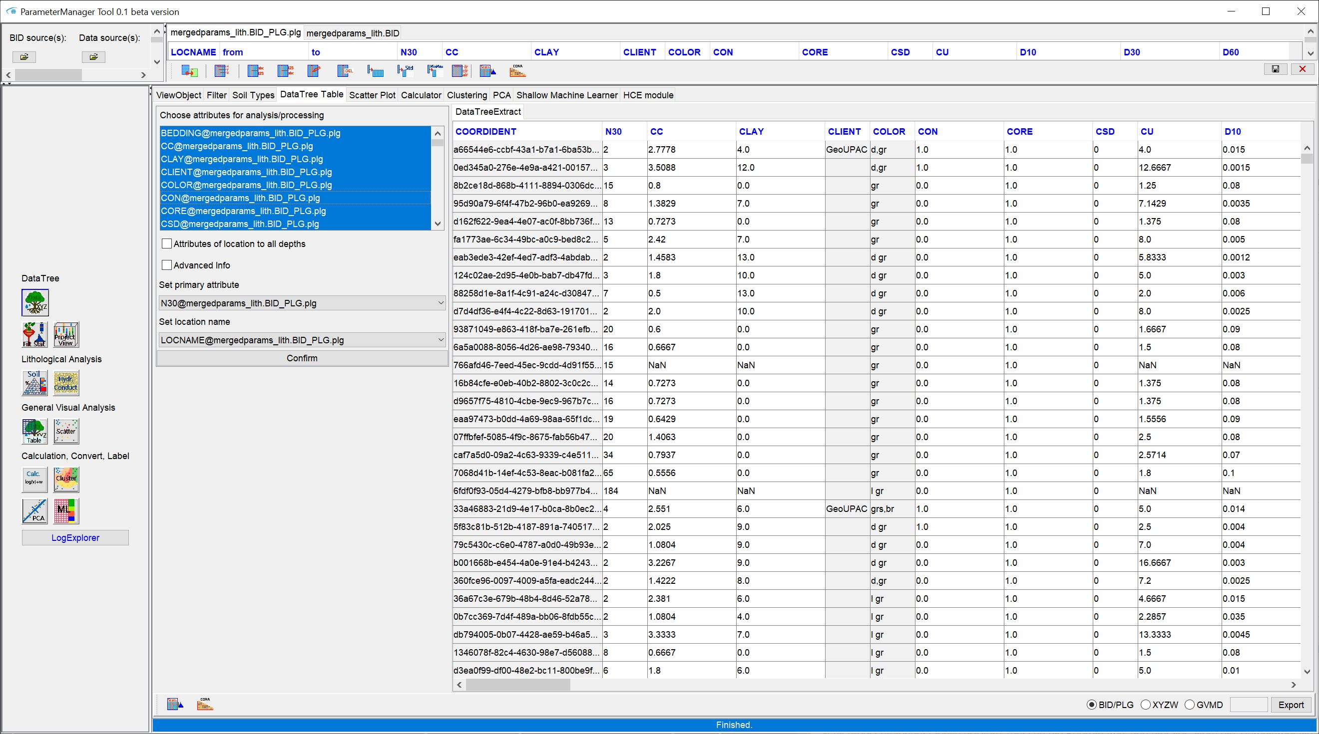
The example of labelling layer descriptions is used to explain it:
We assume that you have a table with the coordinates and depths of a certain marker horizon externally or from the SuburfaceViewer. You have loaded a table with layer descriptions (*.blg) and the corresponding master data (*.bid). Since the labelling was done independently of the layer description table, the coordinates, and the depth intervals, of the labels do not necessarily have to coincide with the coordinates of the layer descriptions. This happens especially if the label originates from a geological conceptual model, where perhaps not all archived boreholes could be taken into account, or where roughly recorded borehole data were neglected, or new boreholes have now been added, or the modelling took place on a completely different data basis (e.g. seismics). You still want to process and analyse your entire data set of layer descriptions with the label in a table. For this, you have loaded all associated tables into the Parameter Manager and linked them. You have also created the data tree. Now you want to add a new column with the label from the external table to the shift descriptions. 1. Select the attributes you want to insert into the new table from the list Choose attributes for analysis/processing in the user interface. Do it with the mouse and STRG. Note that no table extraction takes place if you have not selected anything in this list. You can select everything with a mouse click and STRG+A.
2. With Attributes of location to all depths checked, you indicate that you want to see location attributes, such as metadata of the borehole, also for each entry with depth interval associated with the borehole.
3. With Advanced info you get further information about the intersection of parameters, e.g. whether there are several entries of a parameter at the coordinates with the corresponding depth interval and the result is a combination of these.
4. With Set primary attribute you define the attribute to which all other parameters are to be intersected. This point should be considered carefully. If there is no information about the primary attribute at a coordinate with a depth interval, no other parameter will be displayed in the output. The primary attribute is geometrically indicative. In our labelling example, you can select the layer description itself (if necessary "Original") as primary attribute, then the intersections with the label depth intervals at matching coordinates are used to assign the label. In the opposite case, the layer descriptions would be assigned to the label, i.e. gglf.s you get a certain number of layer descriptions for a label depth interval, which are combined in one column.
5. Confirm to start the table extraction. Depending on how many different tables and layer entries you have loaded and how many attributes you want to extract, the blending process may take some time. You will see a table with the coordinate ID in the first column, followed by the primary attribute and all the parameters blended with this attribute. You can use this table directly in all other functions of the Parameter Manager, for example for a scatterplot display or a clustering procedure. You will always find the table under the title DataTreeExtract for selection. You can do descriptive statistics and a correlation analysis.
You can export this table. For this, you will see three options to choose from in the lower right corner of the user interface.
By default (BID/PLG) you export the result of the extraction in two files in *.bid- and *.plg-format. This is the usual SubsurfaceViewer format for parameters, which you already know from the Project Settings.
Note that the *.bid file has been generated from the dataset and the Z-values always correspond to the highest detected value at the site. Depending on which primary attribute you have chosen, this may no longer correspond to the drill approach elevation of your original layer description dataset.
Use XYZW to export the dataset into a format usable for 3D IDW interpolation or 3D kriging estimation. This export includes a vertical gridding, the step size of which you enter in the text box on the right. This is advantageous because it allows you to bring parameters defined by irregularly long depth intervals into a vertical density suitable for interpolation.
With GVMD you export the contents of the extracted table into an irregular voxel model. When doing so, enter the value of the maximum XY extent of the voxels on the right. If the primary attribute has a text data type, all voxels have the same XY extent. If the primary attribute is numeric, the horizontal voxel extent is scaled to the parameter that high values are represented by wider voxel columns and low values are represented by narrow voxel columns. The depth intervals are transferred unchanged in the irregular voxel model. Voxels in irregular voxel models are allowed to interpenetrate.
¶ Scatterplot
 You can use the Scatterplot function without a data tree, because it only uses tables.
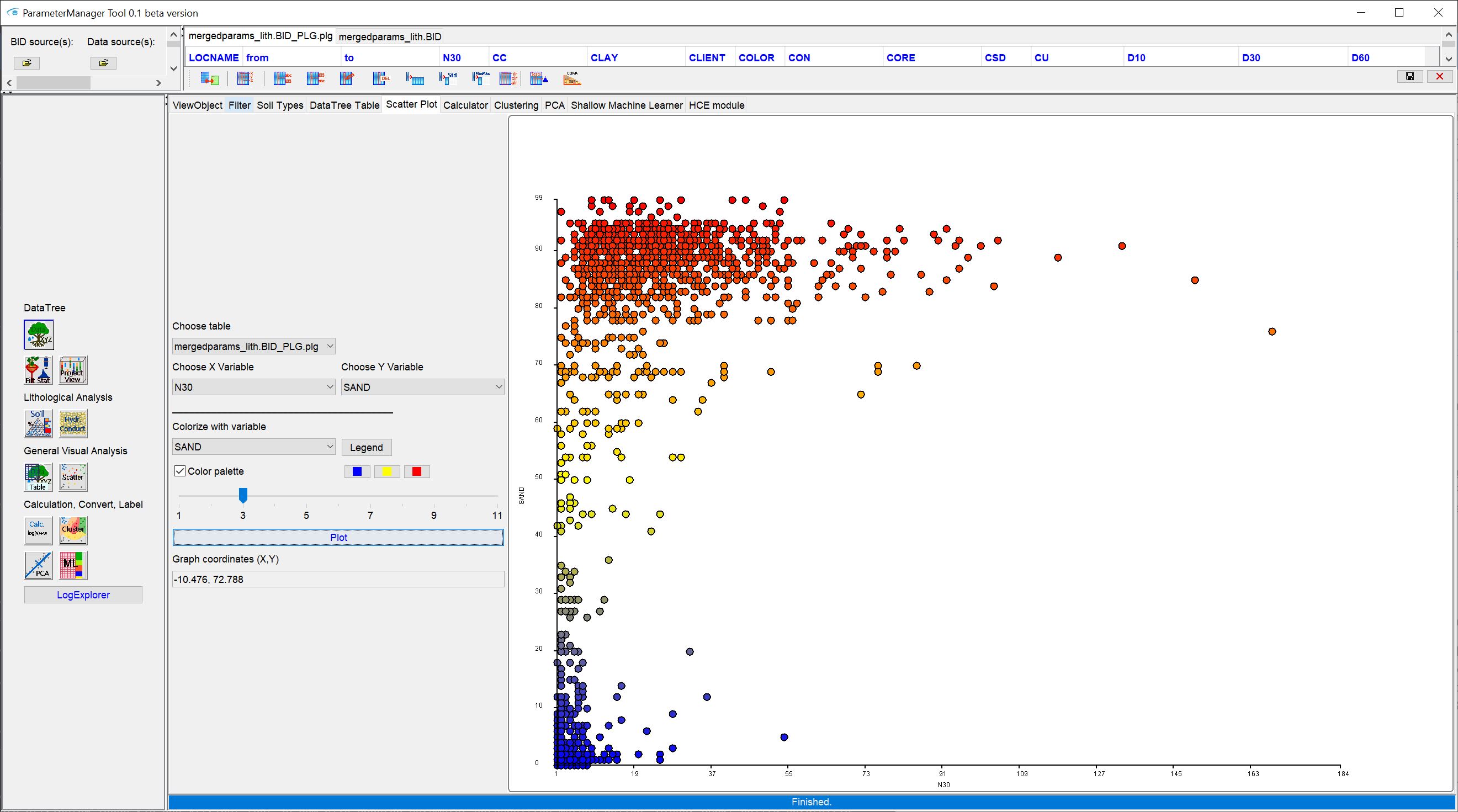
For a scatterplot, use Choose table to select a table that you have loaded or created with the table extraction tool. This fills the dropdown lists for the X and Y variables of the scatterplot with the names of the numerical data series from the table header. Under colorize with variable you see the complete list of the header line, except that you select the colouring variable. You can define the colours for this variable in three parts with the color palette below or define a legend for this variable via Project View. If you select the variable COLORS from the parser for layer descriptions, the points are displayed in the translated sediment colours. A data series in the same format, and created externally, can also be used here.
Use the slider below to set the point size in the Scatterplot.
Confirm with Plot and the graph is completed on the right-hand side. For better orientation in the plot, move the mouse over it and read off the data of the x- and y-axis under Graph coordinates.
Note: You can save the scatterplot. To do this, double-click with the mouse in the drawing. You will be asked to export it as a SVG file. {.is-info}
¶ Calculate, Convert, Label
In this category you will find only functions that are performed on a table basis. This means that you do not necessarily need the data tree to use them. You only need to have tables loaded in the system.
¶ Calculator
![]() This is a calculator with which you can calculate numerical parameters with each other in the Parameter Manager.
This is a calculator with which you can calculate numerical parameters with each other in the Parameter Manager.
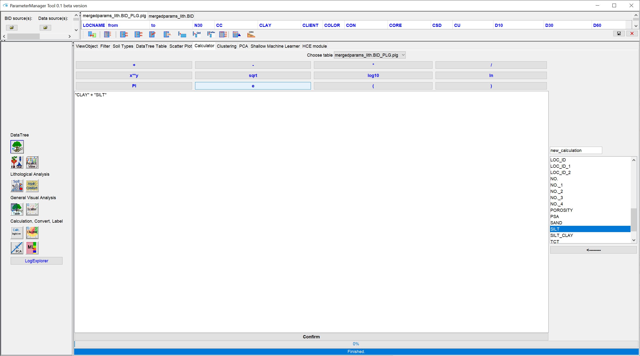
Select the corresponding table in the upper dropdown list. Then select a name for the result column in the text field new calculation. Enter your calculation in the formula window and press confirm to perform the calculation. The result will appear at the top of the new column in your selected table.
It seems to happen from time to time that the new column is not rendered. In this case, save the table. The new column will be present in the saved table. You have to reload this table in that case.
¶ Clustering
![]()
Note: This function uses Python. Allow the Python installation during the SubsurfaceViewer installation. This guarantees that all the required libraries are included. In addition, you should have defined the python.exe path under Program Settings.
With this user interface you can perform clustering on numerical columns of your selected table in a simplified way. An interface and corresponding calculations to determine the most favourable cluster count are integrated. If you are proficient in Python scripting, you can delve deeper into the matter and operate corresponding libraries yourself via Python. In that case you have more setting options. The integration into the SubsurfaceViewer is intended to make it easier to get started and to make the clustering methods accessible to those who do not have the time to deal with Python in depth. In conceptual modelling, clustering makes it possible to quickly and intuitively bundle information, which is a great advantage, especially when the data load is high, in order to obtain an overview and allow the correct interpretations to follow.
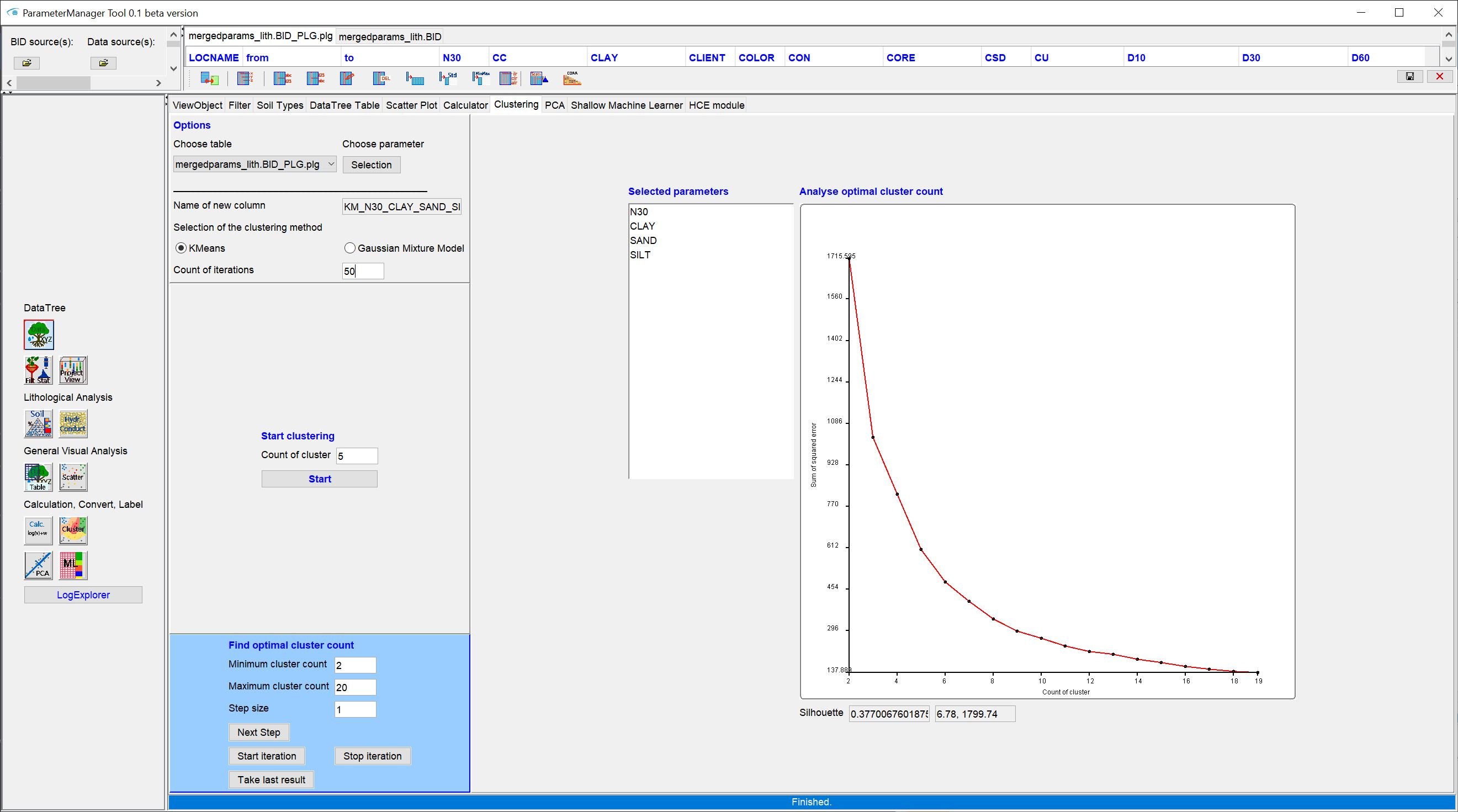
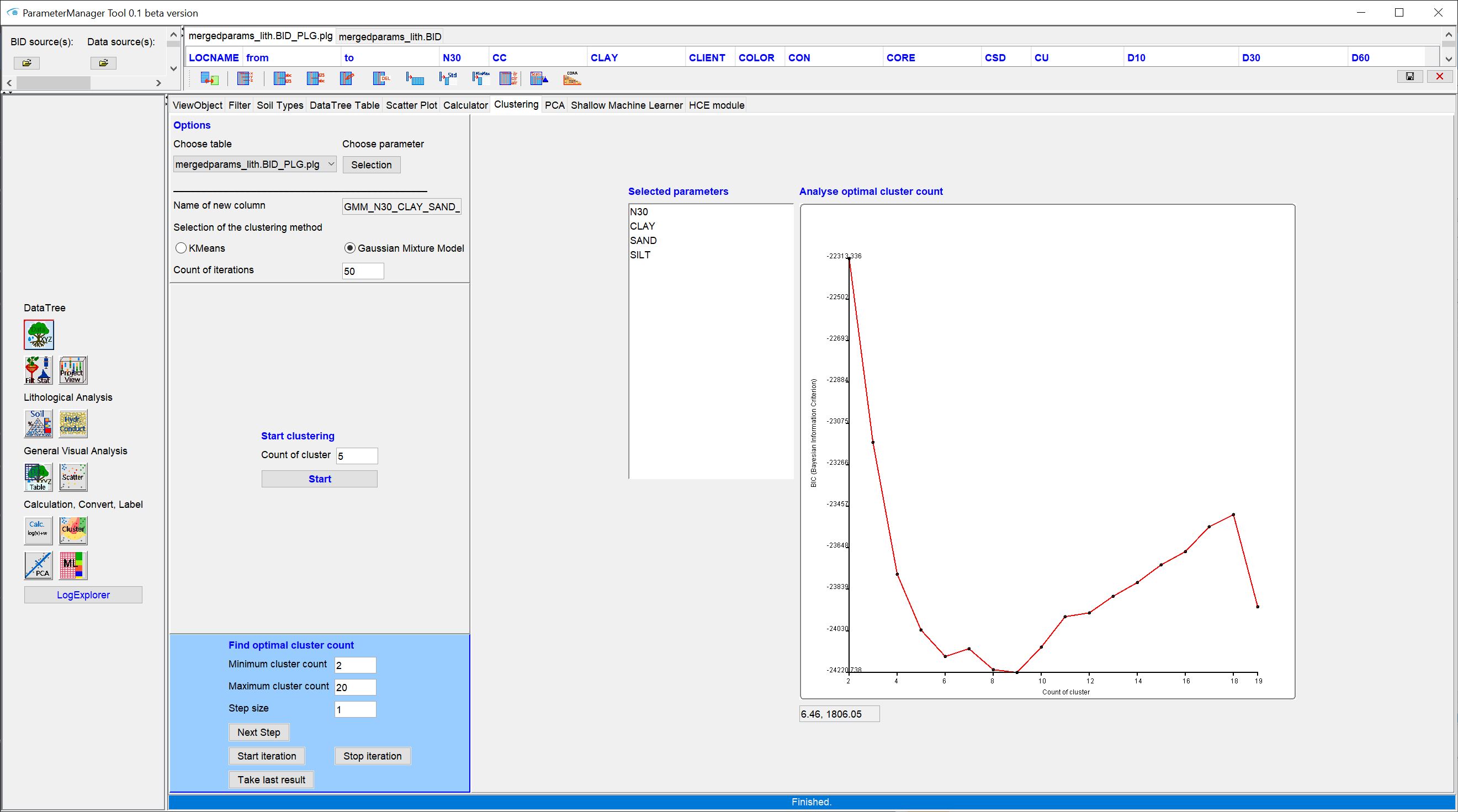
The clustering function accesses the Python library sklearn and uses here either K-means, Mini-Batch K-means or Gaussian Mixture Models. You can select either K-means or Gaussian Mixture Model as the method in the user interface. Mini-Batch K-means is carried out automatically if the data set exceeds a number of 25000 entries. You will be informed about this in the Info window. Gaussian Mixture is performed with the covariance model full. K-means with the algorithm "lloyd". Details on the clustering methods are best obtained from the sklearn pages linked above.
Note: After performing a clustering, read the log in the info-window. Here you can see, whether the algorithm converged or whether there were any problems during the execution.
The user interface is divided into two parts. On the left is the field for the options. Here, you define the general clustering settings in the upper area. In the middle you run the clustering in its final version. At the bottom you see a blue field. Here you can make settings that lead an analysis to the optimal number of clusters. The results are displayed graphically on the right.
Next to the dropdown list for selecting the table on whose contents clustering is to be performed, you will see a button labelled choose parameter -> selection. Here you open a window with a list of the numerical columns of your selected table. Select the corresponding input parameters with a mouse click and STRG and press new selection. The selected parameters are immediately displayed in the centre of the selected parameters list. The name of the output column is created automatically and can be seen under name of new column. A "KM_" at the beginning stands for the result from the K-means clustering. If you have selected the Gaussian Mixture Model method, the name is preceded by "GMM_".
Under the selection of the method (Selection of clustering method) you will find an input field for Count of iterations. There may be slight differences per clustering run with the same settings, as these algorithms start with conditional random starting conditions and then pursue error minimisation through internal iteration. If the determined error has fallen below a tolerance value or can no longer be minimised, the run is completed (the system has converged). This does not mean, that there is no "better" way. On this subject, you can look up "error minimisation", "overfitting" and "underfitting" in machine learning methods on the Internet. You have the option of clustering several times with the same settings in the Count of iterations input field. The system provides you with the best result at the end of the process with regard to the error criterion. In the case of the K-means, this is the so-called silhouette value. The run with a silhouette value closer to 1., is declared the best run. You can find the silhouette value in the log of the clustering in the info-window and below the graph on the right in the small text box. In the case of the Gaussian Mixture Model, both the Akaike Information Criterion (AIC) and the Bayesian Information Criterion (BIC) are calculated. In both cases, a lower value is decisive. For the graphical output and the final selection of the best run, the lowest BIC is sought. This is based on our previous experience. In the info-window you can still see the output of the AIC in the protocol.
If you know the number of clusters you want to see in the result, you can proceed with the field start clustering. Enter the number of clusters in the text field and press start.
Note: The tool uses the temporary directory to store the calculation. You can adjust the path of this directory with the Programme Settings.
¶ PCA (Principal Component Analysis)

**This function uses Python. Allow the Python installation during the SubsurfaceViewer installation. This guarantees that all the required libraries are included. In addition, you should have defined the python.exe path under Program Settings.
With this user interface you can perform a Principal Component Analysis on numerical columns of your selected table in a simplified way. The user interface is very simple. On the left hand side you select the table from whose parameters you want to create a PCA. With the button Choose parameter -> Selection you select the columns of the target parameters from the list with mouse click and STRG and confirm with new selection. The selected parameters appear in the list on the right.
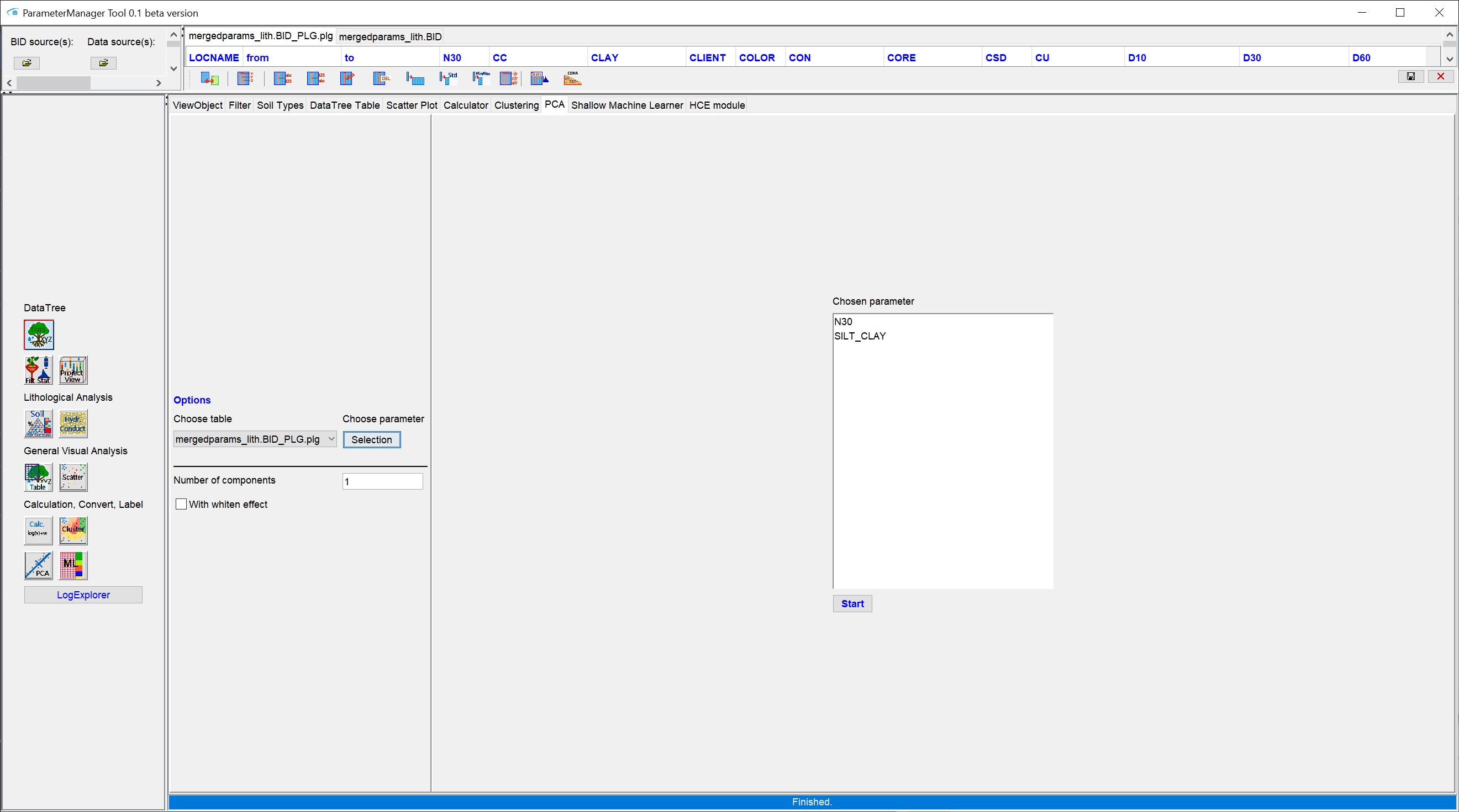
With number of components you set the number of components. This should be smaller than the number of parameters entered. If you enter a component number of 1, basically the information from all selected parameters are reduced from multidimensional to one-dimensional with PCA.
We have used this method in practice to generate downhole curves for automatic multicriteria analysis of sediment properties to depth. We were able to convert RGBA values into a one-dimensional PCA value, creating the equivalent of a "colour curve" that was easier to compare with downhole measurements or lithological curves. PCA is more often used in geostatistical analyses.
The result is stored in a column with the title scheme "PCA_" + "ID of component". You can find more information about the process in the log of the info-window.
Note: The tool uses the temporary directory to store the calculation. You can adjust the path of this directory with the Programme Settings.
¶ ML (Shallow Machine Learner)

**This function uses Python. Allow the Python installation during the SubsurfaceViewer installation. This guarantees that all the required libraries are included. In addition, you should have defined the python.exe path under Program Settings.
With this user interface, you can perform shallow machine learning (ML) classification on numeric columns of your selected table in a simplified way. You can classify here, but not perform regression.
If you have Python scripting skills, we recommend that you work directly on the Python libraries that we have linked to in the title of each user interface. The user interface implemented here is intended to be a support during your modelling for those users who do not have the time or the Python scripting skills available.
Automatic labelling can be helpful in preprocessing and for validating your conceptual model and has been introduced here in a simplified way. We have explained an application example in the article Advanced Classifications.
The user interface is simple. You have the ML methods Random Forest Classification and XGBoost Classification at your disposal, which you activate by pressing the respective buttons in the upper bar of the user interface.
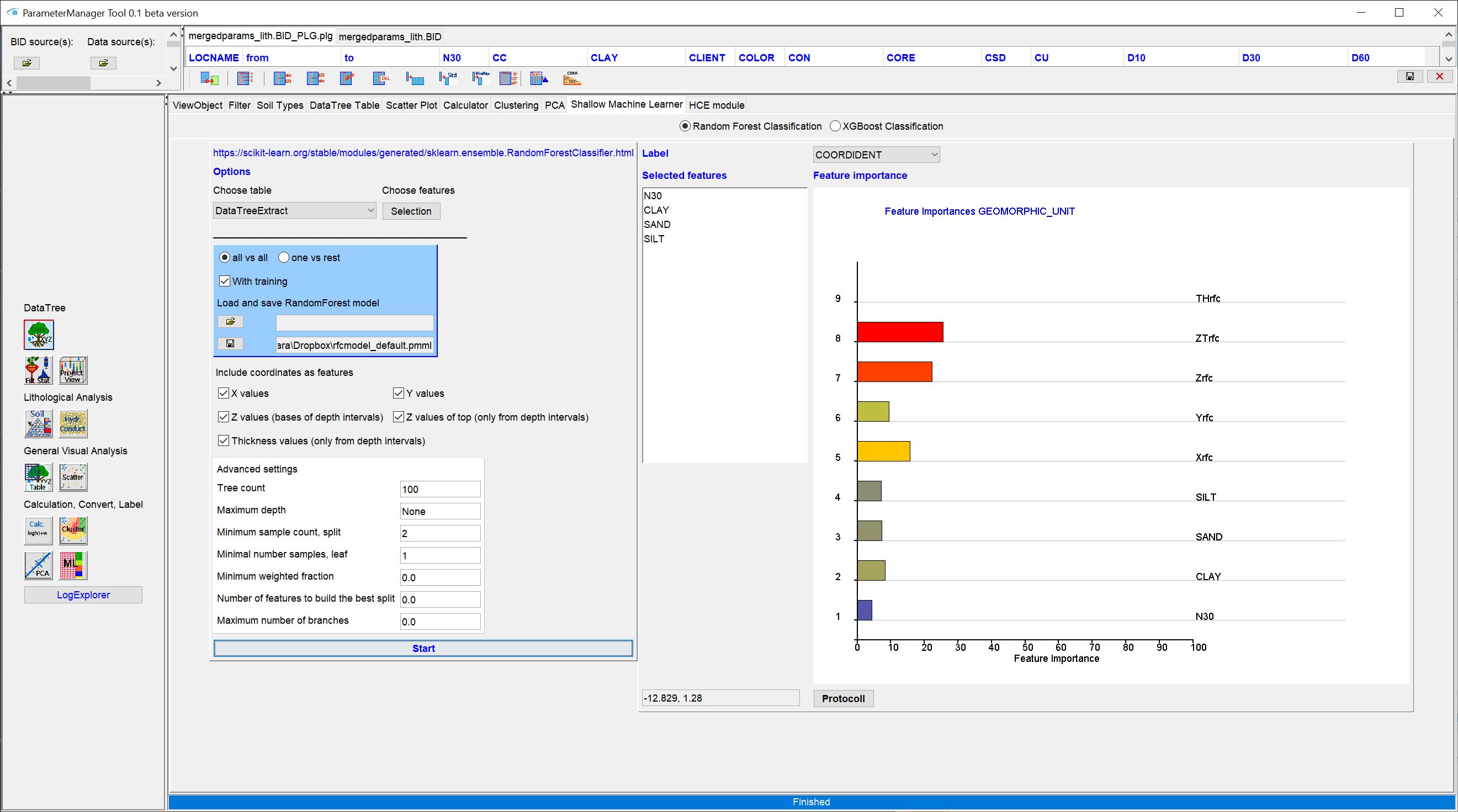
On the left side you see options for the respective methods, as well as storage and loading options for trained models. On the right side you see the selected parameters, the selected label to be trained with, a graph of the feature importance and a button with which you can read the protocol of the Python process again as text and copy it.
Left side:
Under Choose table you select the table you want to use for classification or labelling. This can be the DataTreeExtract, a table that you have already extracted from a data tree. With Choose features a small dialogue opens that lists the numeric columns of your selected table. Here you select the parameters you want to use as features with a mouse click and STRG.
In the blue field below you have the possibility to modify the labelling. With all vs all, all labels used for training are tested against all others. This setting can be selected without training (With training) in order to use an already trained model for the labelling of an unknown data set. When the process is completed, there are two columns with the most probable label as the result of the estimation - once as ID and once as full text. After that, you see as many columns as there were labels, with the IDs of these labels as headers and below that the probability of occurrence that the machine estimated for these labels. There are numbers between 0 (not at all likely) and 1 (100% likely). With one vs rest you have a special option that is used for a validation of a conceptual model. This setting can be used in training mode (With training is active and there are already labels in your table). If you activate one vs rest, you will see a dropdown list showing the contents of the uniform words of your right selected label. If you select a word, the label record will be binary coded, i.e. items containing the word shown in this dropdown list as a label will get a 1 and all others will get a 0. You trigger the machine to give a Are you...? Yes or No response. Under this condition, if you look at the feature weights with solid estimation (cross-validation is fine), you should see the rules of thumb used to distinguish this label from others reflected. In this way, unknown or previously undiscovered sets of rules can possibly be found through the processing of third parties. It can also serve to summarise and check one's own qualitative uncertainty of the assessment that led to the respective label (e.g. geological layer affiliation from a conceptual model) by means of the probabilities of occurrence for the answer Yes/No in a number. We have provided a corresponding practical example for you in this article.
If you have selected the DataTreeExtract-Table, you will see boxes under the blue field that you can check and uncheck. Since this table comes from the data tree, it is certainly georeferenced and already checked for duplicates. You can integrate the coordinates as well as the depth intervals and their thickness as features into your machine estimation. If you have selected any table from the parameter manager, these fields will not be displayed.
If Random Forest Classification is active, you have the possibility below to set extended settings according to the sklearn library for the Random Forest algorithm. We have made the meanings and input options available to you as short versions in tooltips for display.We recommend that you read up on this again on the link given above the options. We have integrated the standard settings of Random Forest Clasification in the text fields as a suggestion.
For the user interface of the XGBoost Classification, we have omitted in-depth settings for simplification.
When your estimation is complete, you will see the resulting *Feature Importance in the graph. They always add up to 1, i.e. you see the importance of individual features compared to others in order to arrive at the corresponding label. If you want to save this graphic, you can double-click with the mouse in the graphic and you will be offered to save an SVG file.
Note: We always use 75% percent of the labelled data set for training. The other 25% is used for validation. We estimate the entire data set with the "trained machine ", i.e. the labelled and the unlabelled data set. This way you can compare the labelling with the original labelling. If you analyse this with the log and the resulting feature weights, you can get a better estimate of the quality of the estimation, the quality of the label or the suitability of the selected features and make appropriate improvements.
The saved trained models are saved as PMML in the case of the Random Forest Classification tool; in the case of the XGBoost Classification tool, the *.xgboost format specially tailored for this algorithm.
Note: You can save a trained machine and load it again for a new training or use it for an unknown data set. Always document the label variable used and the features selected for your stored trained models to not get confused. The SubsurfaceViewer will check whether the number of features used still matches the number of features present in the trained machine. Otherwise, an error message will be issued here.
Note: The tool uses the temporary directory to store the calculation. You can adjust the path of this directory with the Program Settings.
Sometimes the table used, especially DataTreeTableExtract does not seem to render the newly created columns. Then you should export the table. You will see that the columns have been added and only the rendering has not been updated.
¶ LogExplorer
At the very bottom you will find a button to open the LogExplorer. Since this is somewhat more extensive, we have written a separate article on this.