The LocView Object is part of the Parameter Manager, which you will find via the main menu bar under Tools -> Advanced Tools -> For parameter. You should be familiar with the Parameter Manager in order to be able to create a LocView object.
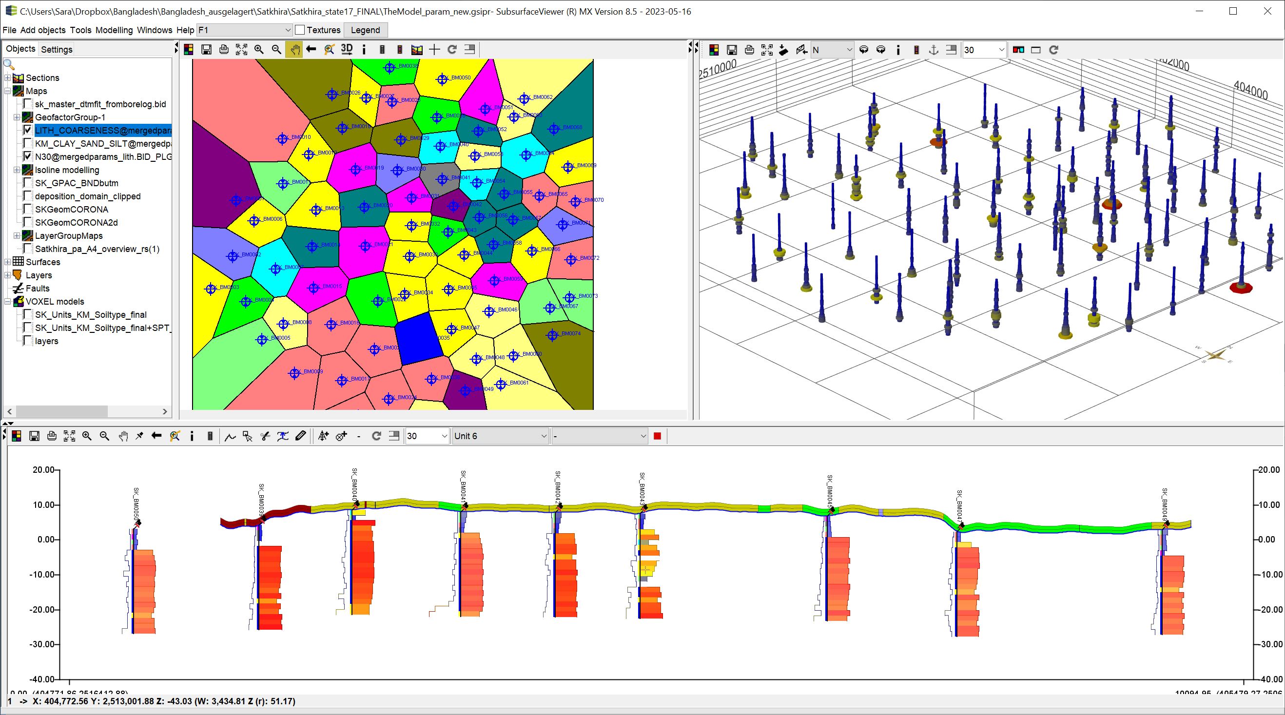
The LocView object is similar to the Drillings with or without parameters (e.g. via *.plg or LAS files) in the SubsurfaceViewer, but is specialised in reading parameters of any geometric description from tables, analysing, filtering and further processing them. Numerical data can be displayed as curves, filtered if necessary, in the sections and in the 3D view. Descriptive data are displayed as variably adjustable columns. Voronoi maps can be calculated directly under query conditions and you can create colour gradients.
The LocView object has a direct connection to the LogExplorer.
LocView objects cannot be integrated into the section like Drillings (read the article Construct Profile Sections). You must set a buffer distance to the profile sections in the Settings of the object. All objects with XY coordinates within this buffer distance are projected into the profile sections and faded in.
If you have created a LocView object, it appears in the object trees under the category Maps. It receives the name of the parameter to be displayed linked via an @ symbol with the short name of the source table in the Parameter Manager.
Background Information:
Each LocView object created is a representation variant of a single underlying data object, which the Parameter Manager creates and manages with the Data Tree. If you filter data in the Parameter Manager, all LocView objects you have displaied will visualise this selection. Each LocView object can be set to display a different parameter at any time via the settings and will change its name in the object tree. The order of the LocView objects in the sections during overlay depends on the time of their creation. The last LocView object overlays the first one. {.is-info}
¶ Generate LocView Objects
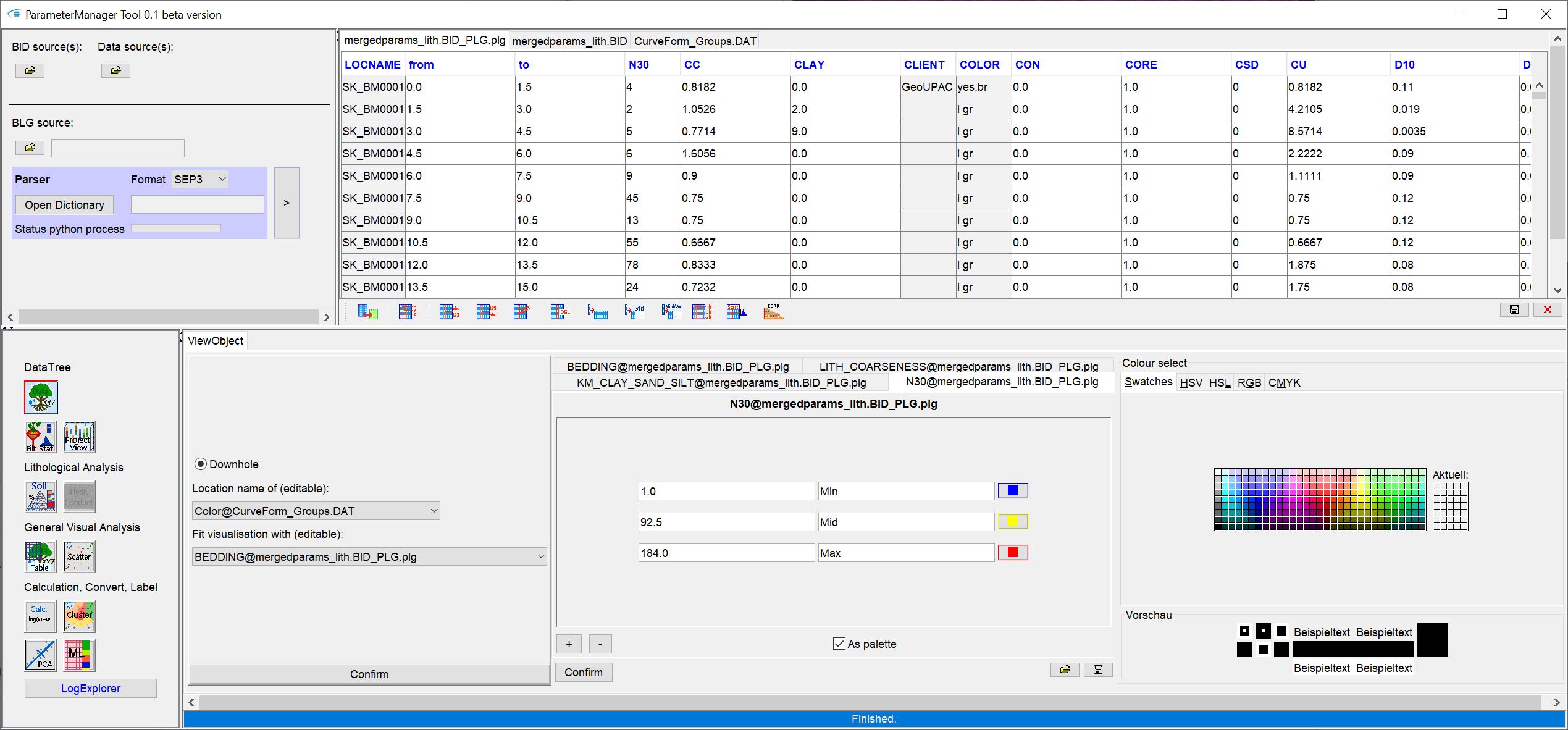
Open the Parameter Manager. Use the button ![]() for Project View in the section at the bottom left. The corresponding user interface will open on the right side in its own tab. As soon as you have selected a parameter with the Dropdown list Fit visualisation with (editable), a legend editor appears on the right. The user interface for this is structured in the same way as the centrally available legend editor. There can be several legend editors, which are displayed in tabs for each parameter. The legends are initially created automatically based on the data distribution of the selected parameter. You can subsequently modify or process the legends in the formats as we have summarised for you in this article.
for Project View in the section at the bottom left. The corresponding user interface will open on the right side in its own tab. As soon as you have selected a parameter with the Dropdown list Fit visualisation with (editable), a legend editor appears on the right. The user interface for this is structured in the same way as the centrally available legend editor. There can be several legend editors, which are displayed in tabs for each parameter. The legends are initially created automatically based on the data distribution of the selected parameter. You can subsequently modify or process the legends in the formats as we have summarised for you in this article.
Note: If you have ever used parameters to colour Scatterplots, Ternary diagrams or in LogExplorer, legends may have been generated automatically. With an operation of the Dropdown list you update the tab view of the legend editors. You will see all the legends that have been automatically created to that point in the tab.
When you save a project with Data Tree and a LocView object, the Parameter Legend is also saved.
Select the name that the locations should be shown in the 2D view through a possible Location-Labelling in the Dropdown list Location name of (editable) .
As soon as you Confirm a new LocView object is displayed in the Standard User Interface under the cateogy Maps. In the 2D-View you will see symbols for the locations. In the section and in the 3D view you see your parameters, depending on the setting, as columns or curves.
Note: When you create the first LocView object and there are several hundred thousand coordinates in the data tree, it may take some time to create the object. Since all LocView objects refer to the same data object, you do not have to wait long when creating all other LocView objects. {.is-info}
¶ General Options
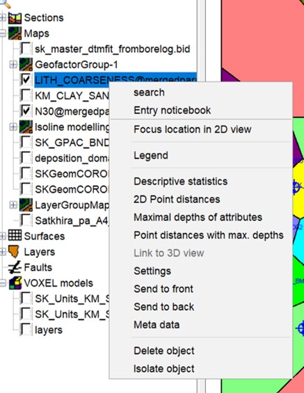
You can read about the options here.
¶ Focus location in 2D view
These options are the same like the [Boreholes-Options](/en/Funktionen/Bohrungen#center-borehole-in-2D-view).
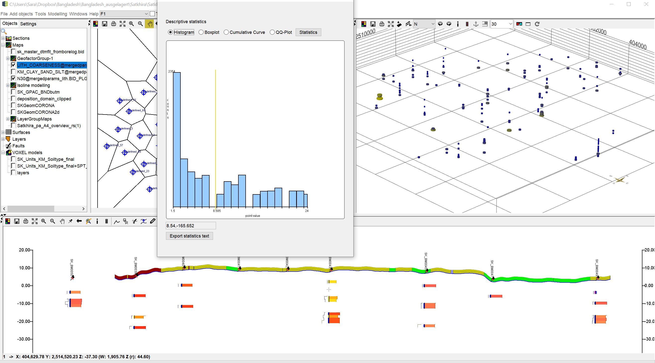
¶ Descriptive statistics
This shows the descriptive statistics for the parameter currently displayed. If you have a Filter activated, the filtered data will also be evaluated.
¶ 2D point distances
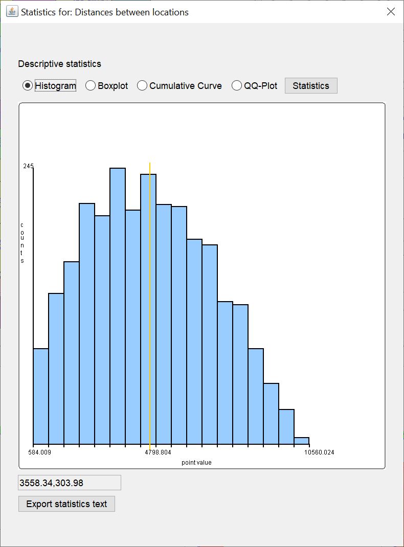
Here you can view the 2D point distances of the data points of the LocView object currently displayed as statistics. If you have a Filter activated, the filtered data will also be evaluated.
¶ Maximal depths of attributes
The maximum depths (under terrain) of the data points of the LocView object are currently displayed as statistics. If you have a Filter activated, the filtered data will also be evaluated.
¶ Point distances with max. depths
The 3D point distances using the maximum extension of the depth intervals of the data points of the LocView object are displayed as statistics. If you have a Filter activated, the filtered data will also be evaluated.
¶ Settings
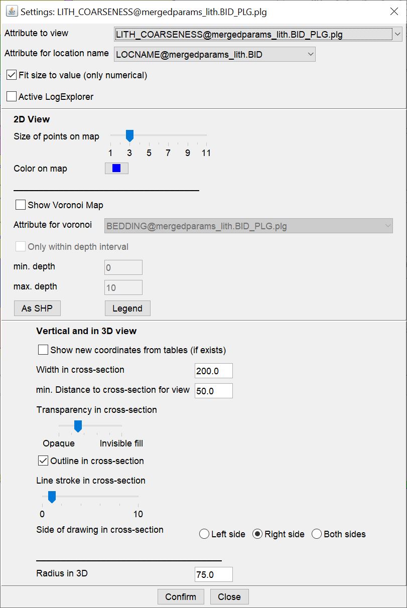
With Attribute to view you select the parameter to be displayed from the dropdown list. These are the 3D parameters with depth interval in the Data tree.
With Attribute for location name you select the parameter from the Dropdown list that is to provide the location name. These are the 3D, more rarely 2D, parameters in the data tree, i.e. without depth interval.
With a tick at Fit size to value (only numerical) you determine whether you want the numerical parameters to be displayed as a curve in the cross-section view and 3D view. Look at the picture at the top of the text to get an impression. If you keep the tick inactive, straight columns are displayed. It is the same when you select parameters with text data type for display. These are shown as columns and the tick at this point is irrelevant.
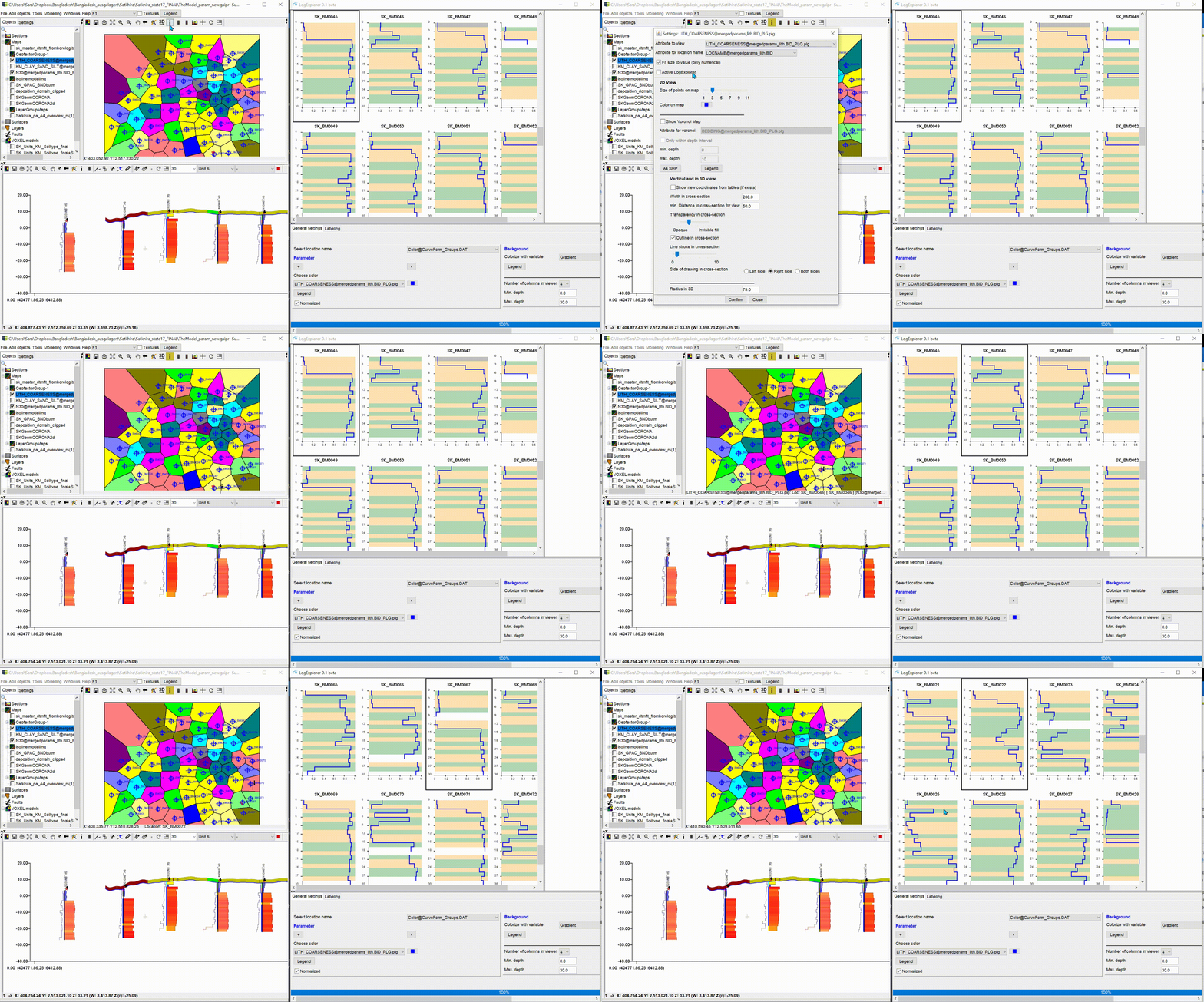
With a tick at Active LogExplorer you can couple the LocView object with the display in the LogExplorer. Click on the location with the  -button and in the LogExplorer, the corresponding window jumps to the picture that belongs to it and frames it in black. This way you can view the data curve with its concrete values. In the LogExplorer you have to deactivate Normalized. If you have created groups in the LogExplorer, you have to make sure that you have the correct group window active on the right, otherwise you will not see the picture of your location. The Voronoi Map, which we describe below, may help you.
The 2D-View settings follow further down. With the slider Size of points on map you change the size of the location symbols in the 2D view and with Color on map the colour.
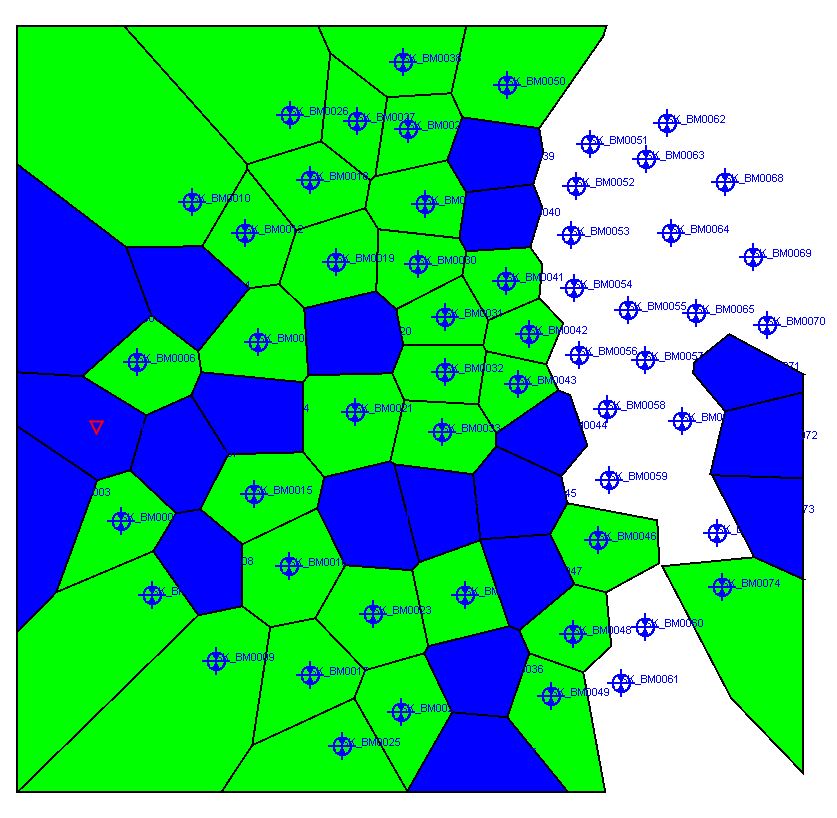
If you check the box Show Voronoi Map, a Voronoi Map will be created around the locations. The polygons of this map receive the information from the parameter selected under Attribute for voronoi. If this is text data with 2D/3D coordinates, such as metadata of a borehole, or groupings from the LogExplorer, the polygons are coloured on this basis. If you click into the polygon in the 2D-View with the  -button, you will get text information below the map. You can view the corresponding parameter legend directly with the Legend button. If you have text data from 3D data with depth intervals, you can have multiple entries. These are strung together with an "&" sign. If you select numeric data, a weighted average is calculated over the vertical based on the thickness and attributed to the polygons.
You can restrict the query of the parameter assignment to the Voronoi polygons to certain depth intervals. Therefore, tick the box Only within depth interval. Enter the target depths under terrain for min. depth and max.depth. If you enter 5 - 10 metres, the weighted mean values of a numerical parameter at the site will be calculated for this depth interval and written into the Voronoi polygons.
Export the created Voronoi map as a Polygon-Shape-File and use it in other GIS systems if necessary.
3D-View-Settings.
.gif)
The option to check Show new coordinates from tables (if exists) is displaied. If you check this box, the positions of your displayed parameters are read from the table in the Parameter Manager. You get to see a visualisation of the fluent coordinates of the Parameter Manager. (In the example, the new positioning is unrealistically distant to show the effect).
The visualisation of the fluent coordinates in the 3D-View can help if you are not sure whether the original coordinates are reliable. This can happen with borehole data from archives, because the measuring technique may have been different. You can change the coordinates in the tables a bit by editing and see if the location seems more plausible for your parameters. Attention: if you create a data tree, the new coordinates will be "frozen".
With Width in cross-section you define the width of the columns of the LocView object in cross-section. In the case of numerical data with curve representation, this width corresponds to the highest value plus a small tolerance width for the lowest value. The specification is to be understood in metres.
With min. Distance to cross-section for view you enter the buffer distance that leads to a LocView object being displayed in a profile section at all. This value is in metres.
With Transparency in cross-section you can set the transparency of the column filling using the slider. If you want to see the outline, you can check Outline in cross-section. The slider below controls the thickness of the outline (Line stroke).
Note: If you set the transparency from invisible fill and activate Outline in cross-section, you will have a similar display as LAS curves at Holes. The values are shown as a pure curve.
Use Side of drawing in cross-section to define the side where you want to see the column. Centre (both sides), left (left side) or right (right side).
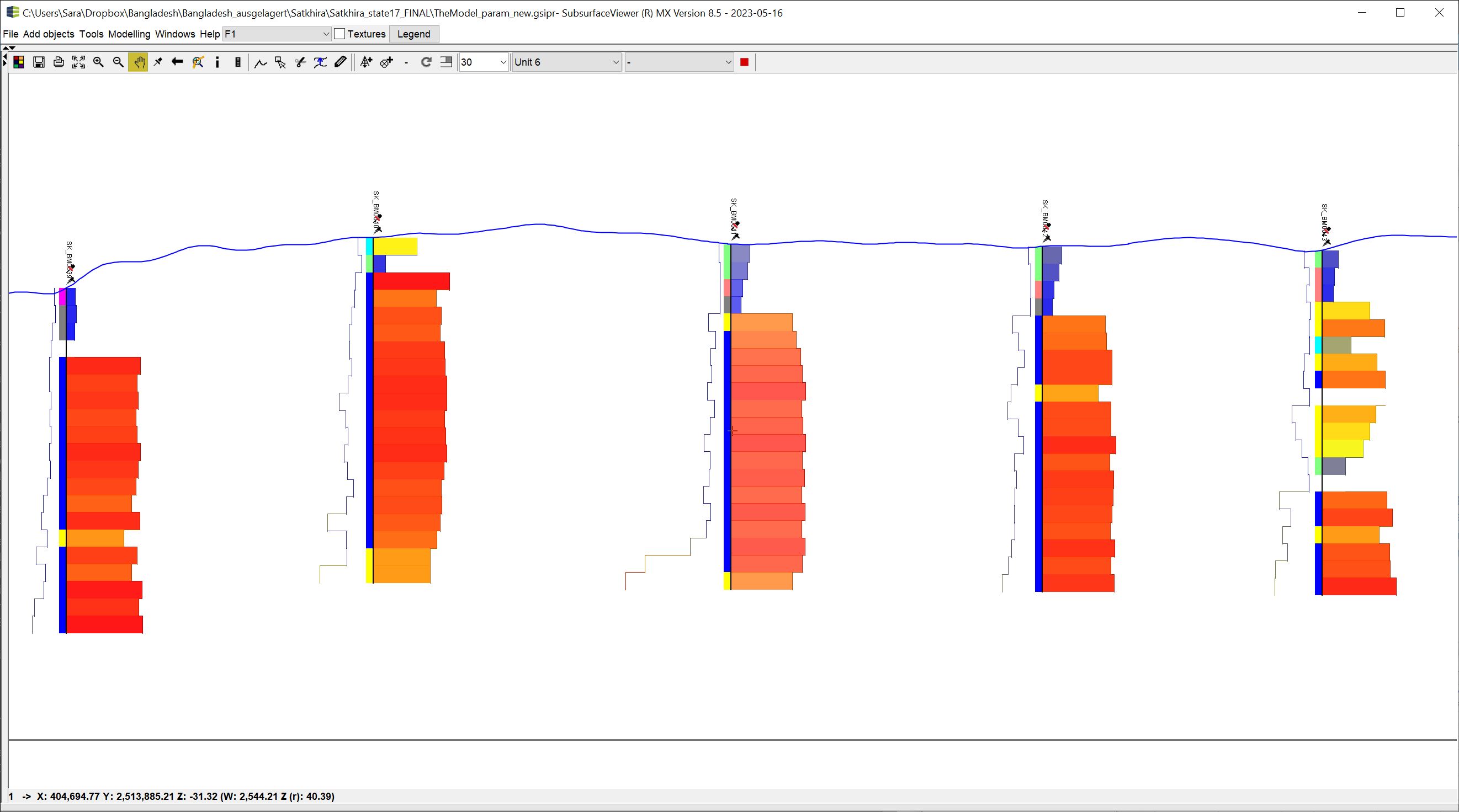
In the example we have brought three LocView objects to display in the profile section:
- One on the right side, with transparent but not invisible column filling, the size of the columns adjusted to the numerical parameter, and an outer line.
- One on the left, with invisible column filling, the outer line and the size of the columns adjusted to the numerical parameter.
- One on the left, with visible column filling, no outer line, significantly narrower columns, and no adjustment of the size to the numerical parameter, since in that case it is an index value.
Use Radius in 3D to define the radius (in metres) of the columns in the 3D view.
Always confirm your settings with Confirm.