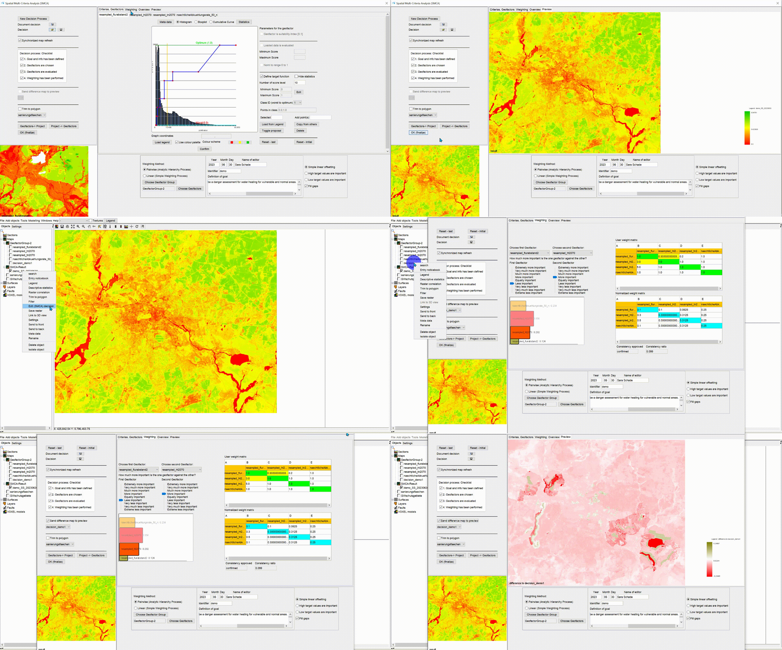
You can find our SMCA tool in the Main Menu Bar under Tools -> Spatial Multi-Criteria Analysis (SMCA).
Note: The SMCA tool only uses raster data (Formats). The output is a suitability map in raster format. If you want to include data from a Polygon-Shape in the decision process, you can use the function Convert to geofactor.
Caution: Closing the window deletes the decision process that is unsaved. Do not close the window until you have been able to add a suitability grid to the project (OK (finalize)) or when you have been able to save the process in an XML file.
In the introduction, we will explain the general structure of this window and then explain the process of a decision-making process with this application step by step using the subchapters.
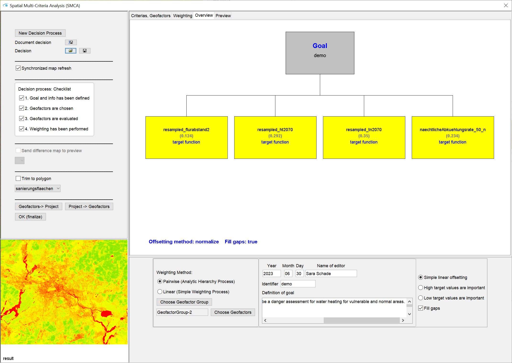
On the left side of the user interface, you will see save and load options for the decision process in the upper field.
With a check mark at Synchronised map refresh, the new result, i.e. the suitability raster, is calculated ad hoc whenever you change your settings. If you work with high-resolution, large raster files, it is recommended to deactivate this check mark that you do not have to wait long for a change. Re-check the box when you want to see the result.
Below you will see a field with a checklist. It cannot be edited directly. The ticks only become active when you have completed all the steps in the decision-making process. Only then you can finalise an event grid with OK (finalize) and add it to the standard user interface.
With Send difference map to preview you can compare your currently created suitability grid with another one by viewing the difference grid for it in the Preview tab (see below). To do this, another decision grid must be in the Standard User Interface. Then select this via the corresponding dropdown list.
With Trim to polygon you can restrict the content of your suitability grid to the inside of a (multi-)polygon. In the Dropdown list, the Polygon shapes invited in the project are listed. If the polygons have been selected in advance, only the selected polygons of the shape are used for the constraint.
The buttons below are explained in the following sections.
At the bottom left you will see a small preview window. Here you can see either the result of the currently set suitability map (result) or, if you are currently evaluating geofactors, the current state of the selected geofactor. More information about this are following.
In the central large field are 4 different tabs:
- Criterias, Geofactors: Here you have access to the rating settings of the loaded geofactors.
- Weighting: Here you determine the weights, i.e. the influence, of the different geofactors/criteria on the decision-making process.
- Overview: The overview shows you a small tree with two levels. At the top you have a box with Goal, to which the Identifier entered below has been passed for an overview. The second level contains a box for each criterion used (geofactor) with its name (black), its current weight (grey) and the type of its evaluation (blue). At the bottom of the window you will see the information of the currently set calculation method (offsetting) and whether gaps are to be filled. You can read more about this in the sections below.
- Preview: Here you can see the suitability grid in its current state, somewhat larger and with a simple value legend. If you have selected Send difference map to preview, you will see the difference map to the comparison grid.
In the lower panel of the window you have to enter the metadata of the decision process and select the criteria (geofactors), the weighting method and the allocation method.
Note: The loaded geofactors are downloaded data from the FIS-Broker of the City of Berlin, especially from the Environmental Atlas Berlin / [Climate Model Berlin] and the Groundwater Flood Distance Map (2009). The evaluations and weighting that we carry out by way of example is not a professional assessment. It does not originate from any scientific or professional background and is only used for presentation purposes of the SMCA tool of the SubsurfaceViewer. Please look at the data directly in the FIS-Broker of the City of Berlin for details and background information.
¶ Start decision process
**All geofactors that are to represent criteria for a decision process must be loaded into the SubsurfaceViewer project with Add objects -> Geofactor raster. An exception arises if you load a decision process that has already been created and the paths for geofactors contained in it are preserved on your PC. Then you can load the decision process file with
.
To start a decision process, open the SMCA window as described above, and enter the metadata for your decision process in the middle, lower input field.
Until you have "touched" each field for the metadata once and entered something, you cannot load any criteria or geofactors for your decision and cannot start the decision process.
The information about who, on what data basis, when and with what objective in mind starts the decision-making process is fundamental content of a decision. Since metadata is often neglected, we have built this restriction into the programme at the request of our users.
A decision-making process is not always simple and unambiguous. Assessments and the assignment of weights to the criteria usually have an individual character. You should be clear about your objective. A description of this in the text field provided can help you to make a decision. But it also guarantees that your peers can better understand your approach and the evaluations. In addition, the decision is also clearly documented.
If the Choose Geofactor Group button on the left has not yet been activated after the last entry in a text field, click with the mouse in one of the text fields.
The checkmark in the checklist Goal and info has been defined is now set.
With the now enabled button Choose Geofactor Group you select the geofactor group you want to work with. An SMCA on a raster basis can only be carried out in SubsurfaceViewer on rasters of the same extension and resolution and therefore only on one geofactor group. For more information read the article on geofactors.
Only geofactor groups with at least two entries will appear in the list. This is because you can only start a decision process on the basis of at least two criteria.
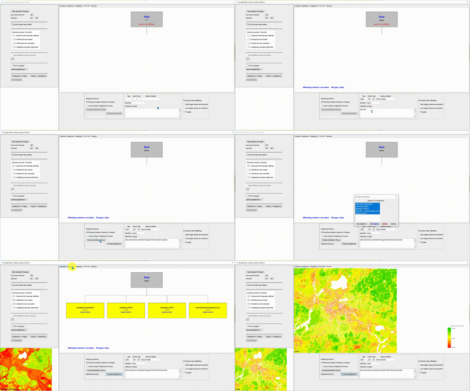
Use the Choose Geofactors button to select the criteria from the list in the pop-up window. To do this, mark the names of the geofactors with a click and STRG. With New selection you define the list of the marked geofactors as a new selection. All previously loaded geofactors are removed from the current decision process. If you select Add objects, the selection in this window is added to the geofactors already loaded. With Delete you delete a geofactor from the decision.
As soon as you confirm, the tree is created or updated and displayed in the Overview tab. In the tab Criterias, Geofactors you will find a separate tab for each geofactor you have added, in which you can set the objective function or the evaluation. You can read more about this below.
The checkmark in the checklist Geofactors are chosen is now set.
If you have activated Synchronised map refresh, a result will be calculated immediately. This only makes sense if you already have evaluated geofactors in the project, i.e. the standard user interface. In this case, this evaluation will be taken over initially. Note that all geofactors have been equally weighted.
¶ Evaluate Geofactors
Note: You need to evaluate geofactors if you use the calculation method Simple linear offsetting. Read about the other two methods in the linked section. Simple linear offsetting is the best known and most used method, as the other two methods are only useful in certain circumstances.
To do this, open the Criterias, Geofactors tab. You will see a separate tab for each geofactor loaded. The tab corresponds to the Settings window of the geofactor. Read the linked article to define a target function or the evaluation contents. Any evaluation initially takes place only in this window.
If you have other target functions in the project, they will not be changed and none will be set in the project from here. This happens when you press the button Geofactors -> Project. Then the evaluation criteria for the geofactors made here in the window are adopted in the project. The button Project -> Geofactors represents the reverse equivalent. The evaluation criteria for the geofactors in the project are transferred to this window.
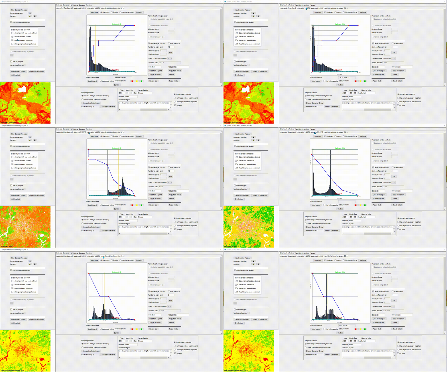
If you select the tabs between the geofactors one after the other, you will notice that the preview in the lower left window changes to the view of the respective geofactor. As soon as you confirm your rating or legend settings, this view will update to the current state of the geofactor currently visible.
If you go out again with the mouse on the general tab for the geofactors, e.g. switch to Overview, you will see the suitability grid at the bottom left with the note result.
The checkmark in the checklist Geofactors are evaluated is set if you have either evaluated all geofactors or you have chosen a calculation method other than Simple linear offsetting.
¶ Determine weights
The weights are numbers between 0 and 1 and add up to 1. They are used to offset the available values of the evaluation from the geofactors at each grid point as a weighted average.
The weights determine the importance of the geofactors on the decision and in comparison to the other criteria.
For this purpose, you can choose between two different methods of weighting in the lower window, which we explain in more detail below.
When you have performed the weighting, the tick in the checklist Weighting has been performed is set.
¶ Pairwise (Analytic Hierarchy Process)
The Analytic Hierarchy Process was developed by Thomas L. Saaty. It is based on a pairwise evaluation of criteria. Saaty said that it is much more difficult to make an almost objective weighting of criteria if they all have to be considered at the same time. He found that people who compare a maximum of two criteria tend to arrive at more consistent weights in a decision-making process and that this can be better understood by others afterwards.
The user interface in the Weighting tab adapts to the theory of the Analytic Hierarchy Process when selecting pairwise weighting.
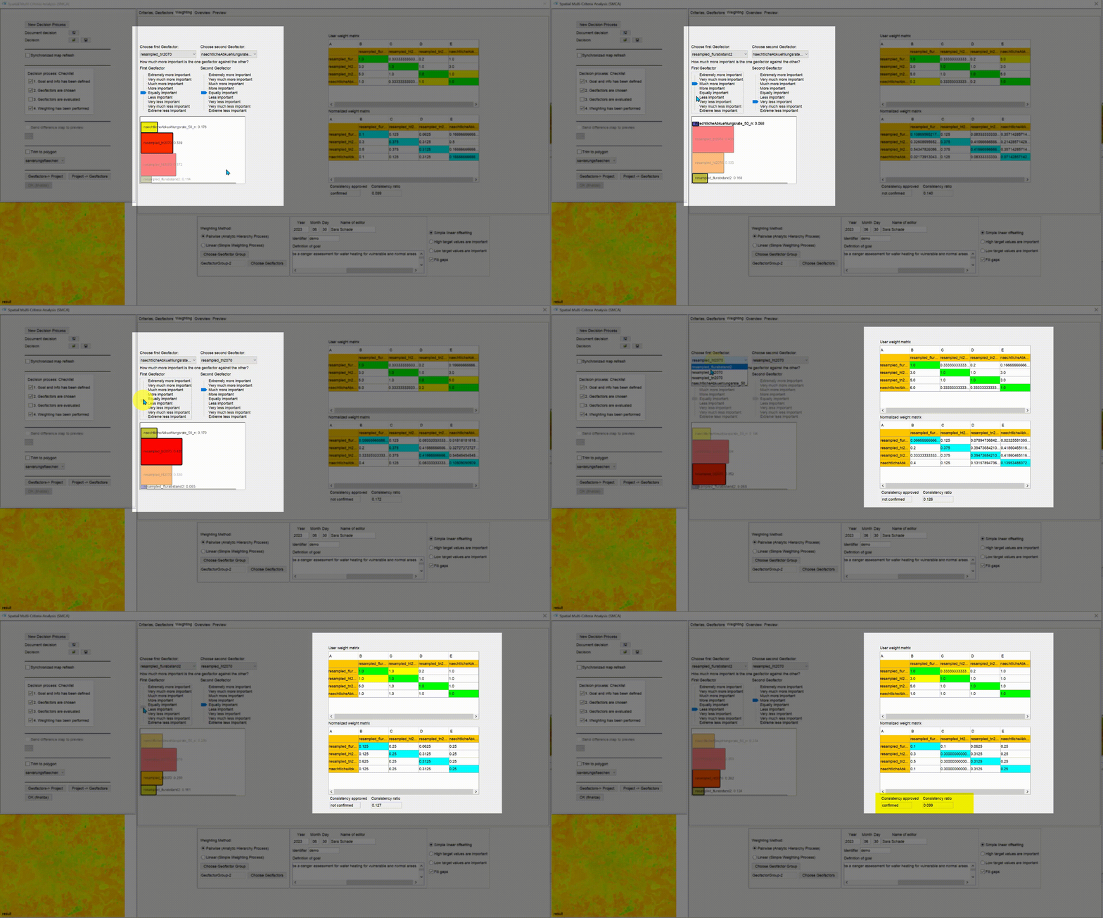
Select the pair of geofactors whose importance for the decision-making process you want to weigh against each other using the two dropdown lists at the top. If you move one of the two sliders to the term that suits you, the other is updated accordingly. The graphic below and the tables on the right are updated.
The two boxes of the geofactors you are currently looking at are more clearly visible in the graphic. The others are "overshadowed" in white so that you can better concentrate on the two current criteria. The size of the displayed boxes reflects the current weight of a criterion in the whole process. This is determined by means of matrix operations in the context of all pairwise weighted criteria.
The determined weights in the overall process appear in the two tables on the right. In the upper table, the weights from the pairwise user setting are shown. Below that, the normalised weights are listed. Read more about the Analytic Hierarchy Process in the literature to understand the entries. If you change the pairs with the dropdown lists, the boxes belonging to the geofactor pair are highlighted in yellow so that you can find them more quickly.
Below the tables you will see the text fields for Consistency approved and Consistency ratio. These two pieces of information help you to make consistent pairwise weightings. A small consistency ratio value is better than a high one. **You can find out whether your pairwise assessment of the weights is conclusive if the field Consistency approved -> confirmed is displayed.
If you save a decision process with a weighting using the Analytic Hierarchy Process, an XML file with the extension *.ahpinfo is created.
¶ Linear (Simple Weighting Process)
A less complex method for determining the weights is the linear variant (Linear (Simple weighting process)). Here you set all weights at once as a percentage value. 100% means that this criterion has absolute importance. A percentage value of 1% reduces the influence of the criterion on the decision-making process to a minimum.
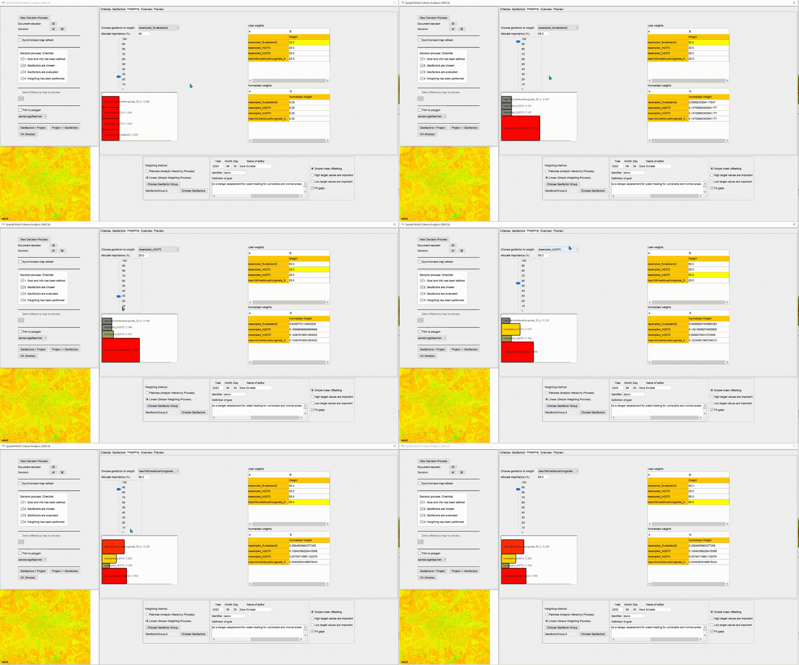
You do not need to worry about the correct weighting, because the weights are standardised in relation to each other so that they always add up to 1. You only need a good feeling to make a correct assessment. So as soon as you move the slider under Allocate importance (%), the entries in the tables on the right and the graph below update.
The size of the boxes shown in the graph reflects the current weight of a criterion in the whole process. The upper table shows the weights actually set by the user and the lower table shows the calculated, normalised weights that will be used in the decision process.
If you save a decision process with a weighting using Analytic Hierarchy Process, an XML file with the extension *.swpinfo is created. {.is-info}
¶ Select Calculation Method
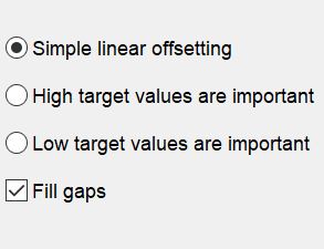
In the lower right options field of the SMCA window you can see the settings for the calculation method.
Simple linear offsetting is the best known and most widely used method. A weighted average is calculated. It is important that the geofactors have been evaluated. No matter which form of scoring you have set, the geofactor scores will always enter the decision process with a value between 0 (worst case) and 1 (best case) corresponding to the score. These values are given the weight you set, which corresponds to a value between 1 (almost not important) and 1 (only important). The result is a suitability grid with values between 0 (completely unsuitable) and 1 (optimally suitable), which is the result of the interaction of the criteria evaluated and their importance assessed.
High target values are important can be used if it is difficult to evaluate geofactors or if it takes too much time. There must be criteria where the highest value of the respective geofactors corresponds to your optimum. The high value for the optimum is not fixed in advance, but results from the value spectrum of the geofactor grids just loaded. Your optimum for the suitability map is reached where there are high values of your criteria everywhere. In the system, this method is generated by dividing all geofactor values to their respective maximum values. Your sought-after optimal values always approach the value 1. All other values that are further away from 1 are further away from the optimal state you are looking for. The range of values can become negative. The result is a suitability map tailored to this particular question, which can reflect relative ratios to the optimal state (~1). Note with this method that a division by 0 is not possible. If the maximum value of a geofactor is 0, you cannot use this method.
Low target values are important can be used if it is difficult to evaluate geofactors or if it takes too much time. There must be criteria where the lowest value of the respective geofactors corresponds to your optimum. The lowest value for the optimum is not fixed in advance, but results from the range of values of the geofactor grids just loaded. Your optimum for the suitability map has reached where low values of your criteria are present everywhere. In the system, this method is generated by dividing all geofactor values to their respective value minimum. Your sought-after optimal values thus always approach the value 1. All other values that are further away from 1 are also further away from the optimal state you are looking for. The range of values can contain negative or very high numbers. The result is a suitability map tailored to this particular question, which can only reflect relative ratios to the optimal state (~1). Note with this method that a division by 0 is not possible. If the minimum value of a geofactor is 0, you cannot use this method.
With a check mark at Fill gaps you can determine how to proceed if a NoData value is set for a geofactor at a certain grid coordinate. If you think that in the absence of a criterion at this location no decision can be made for these locations, you should deactivate the checkmark. A NoData value will appear in the suitability grid. If you want the remaining criteria to be calculated at this location, then set the checkmark. At the location concerned, the weights of the geofactors are updated with data in the correct ratio and the suitability map receives a decision result without the geofactor that contained no data at the location.
¶ Close the decision-making process
Save the decision process. You can do this with  . Here the process is saved in a text format and is available for you to insert into a documentation. If you use the
  symbol, the process is saved in an XML file, which you can load into this window with
  .
.
The ending of the XML file is determined by the selected weighting method. *.ahpinfo -> Analytic Hierarchy Process and *.swpinfo -> Simple Weighting Process. {.is-info}
When the checklist on the left shows all ticks, the button OK (finalize) is active and you can add your suitability map to the project by using this button.
The result is displayed as a geofactor in its own subfolder SMCA-Result in the category Maps in the object tree. The name of this raster results from the metadata for the date, an abbreviation from the name of the editor and the identifier. The default colouring of the result is always a gradient with red for the worst case (=0), yellow for the acceptable case (=0.5), and green for the optimum (=1).
Note: You can change the decision process by opening the right click context menu of the result and selecting Edit (SMCA) decision. An SMCA window will open for this suitability grid, which is valid for this object. You can create another decision process and run several processes side by side.
If you want to compare your result with a colleague's decision process, you can load it as XML into the general SMCA window and insert the result grid from the loaded process into the project or insert the result as a geofactor externally and open the SMCA window on your result. Both rasters you want to compare should have a check mark in Geofactor is suitability index [0,1] in your Evaluation settings. You can create a difference map of the two rasters under Send difference map to preview. The prerequisite is, that the two result rasters have the same dimension and resolution. It is also advantageous if you have used the calculation Simple linear offsetting.
