Note: The applications described here have been developed within the framework of specific project questions and have not yet run a broad test phase, which is why they are marked with beta status. Please check your results. It is very helpful for us and other users if you give us feedback when you discover a bug.
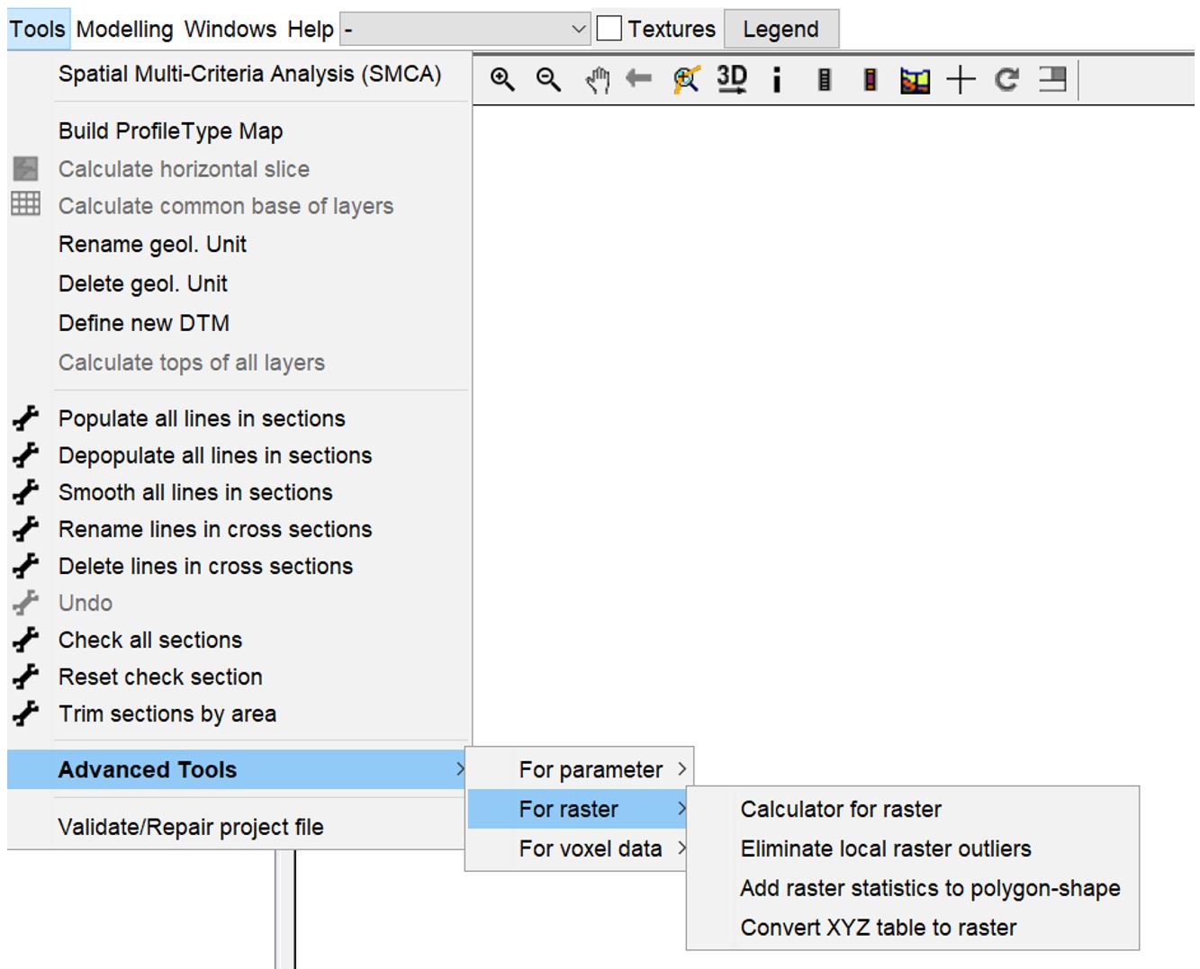
The advanced functions for raster can be found in the menu Tools/Advanced Tools/For raster:
¶ Calculator for raster
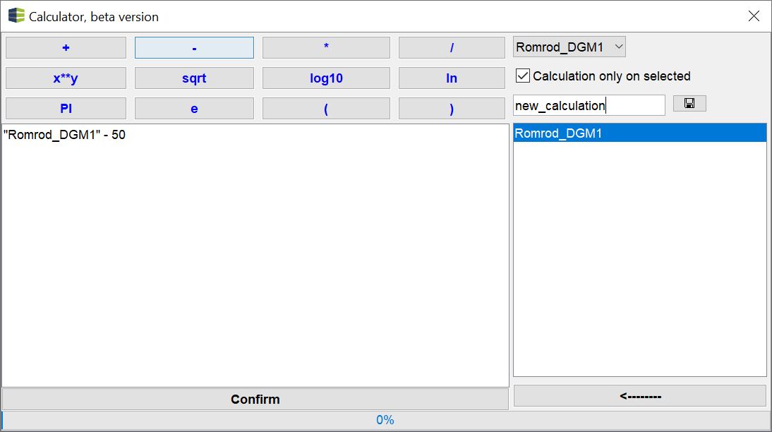
With the calculator for rasters you can make simple calculations on the raster data. Use the dropdown menu at the top right to select one of the raster objects loaded in the project. If there are several rasters with the same dimension and resolution in the project, they are displayed together in the list on the right for calculation. Once you have entered your formula, you must press confirm to perform the calculation. To save, use the diskette symbol at the top right.
With the check mark calculation only on selected you have the possibility to work on filtered data. An example of using the calculator and filter for raster data in combination can be found here. You should note that if you use the filter more than once for different calculations, a temporary file will be written with the name from the text field in the upper right corner. You should not change the name in such a case. There should be enough space in the folder for temporary files. You can define this folder with the programme settings.
In the image below, 50 is subtracted from the filtered data set. Since it is a digital terrain model, the result in the selected area is a surface that is exactly 50 metres below terrain. You can see that the variables, i.e. selected raster data, must be written in the formula with inverted commas.
If you use the button ... or double klick on the name on the list, quotation marks will be set automatically.
¶ Eliminate local raster outliers
Here you can examine a raster for local outliers and smoothing them out accordingly. You can do this on continuous or classified raster files:
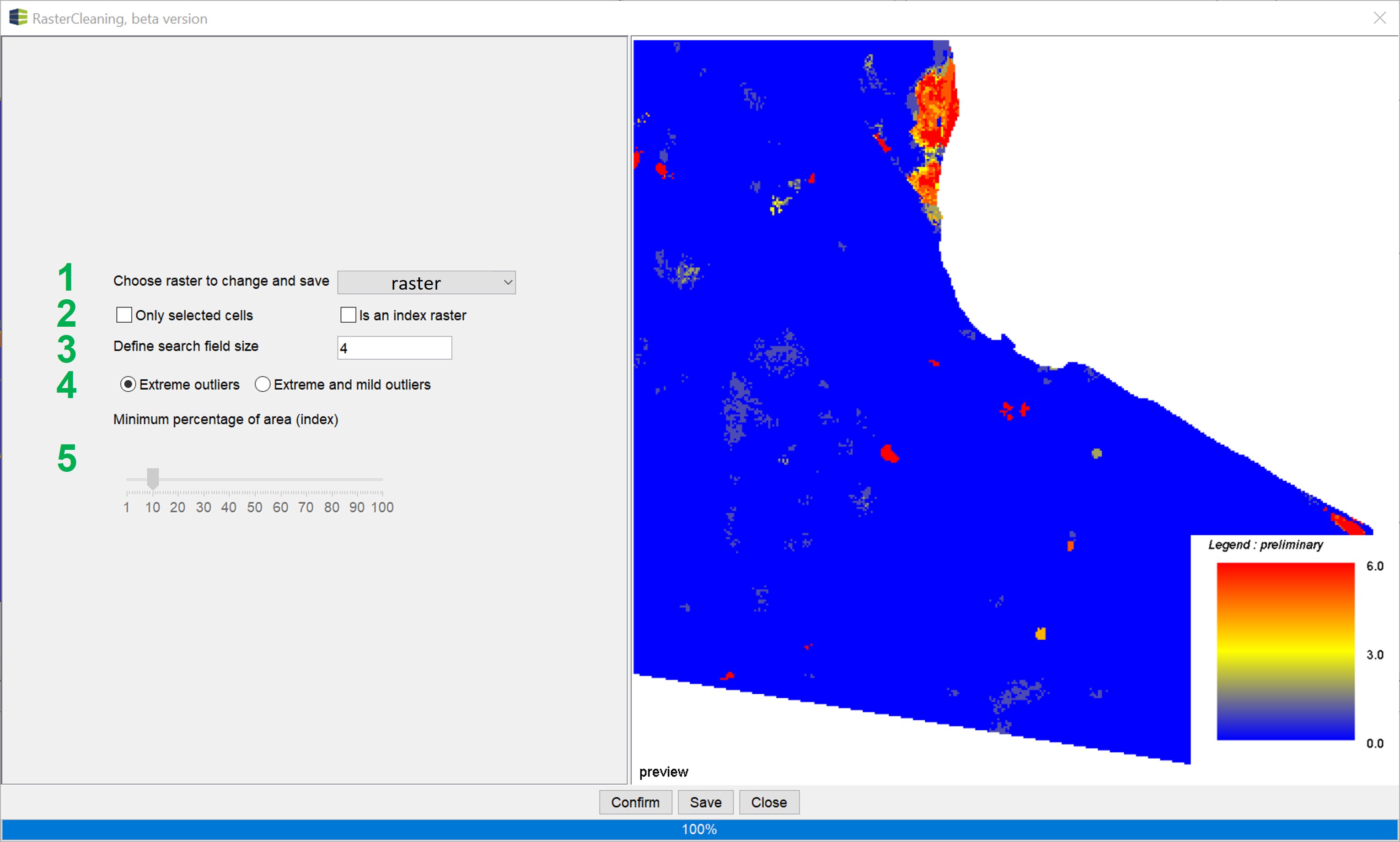
- Use the Dropdown list to select the raster from the project that you want to edit.
- Here you determine whether the clean-up is to be carried out on the entire raster or only on the filtered raster areas (only on selected cells). If you are working with a classified index raster, you should check the is on index raster box.
- Here you define the search field size in which the conditions for a clean-up are set and performed. It names the number of cells around a cell to be calculated and in each direction. A search field size of 10 means that values from 10 cells to the left, 10 above, 10 below and 10 to the right of the target cell are examined together to identify the value of the target cell as an outlier. Cell values that do not represent an outlier remain as they are. 4. If it is not an index grid, you can choose between smoothing extreme outliers (extreme outliers) or mild and extreme outliers (extreme and mild outliers). In this case, a local robust statistic is created in the search field area. Values outside the interquartile range are defined as outliers. Extreme outliers are outside the distance between the interquartile range and 1.5 times the interquartile range. If a value of the target cell is defined as an outlier, it is set to the value of the lowest or highest limit of the outlier consideration. If you have selected the setting extreme and mild outliers and the value is above the upper interquartile range limit, the value is set to the upper interquartile range limit.
- If it is an index grid, the slider is active. With the slider you determine from which percentage threshold of the search field size an index is recognised as an outlier. For example, if you set the slider to 10%, indices that occur in less than 10% of the search field size are set to the index with the highest proportion in the search field. This way you can eliminate individual local indexed grid values. This makes sense, for example, if a classified raster is to convey simplified understanding in further geoinformation systems of the application (e.g. suitability maps) or if calculation artefacts are to be eliminated for this purpose.
Note:
Please note that depending on the resolution and search field size, cleaning up the grid may take some time. It is therefore advisable not to make this calculation in the project currently being edited, but to open a new SubsurfaceViewer window for this purpose.
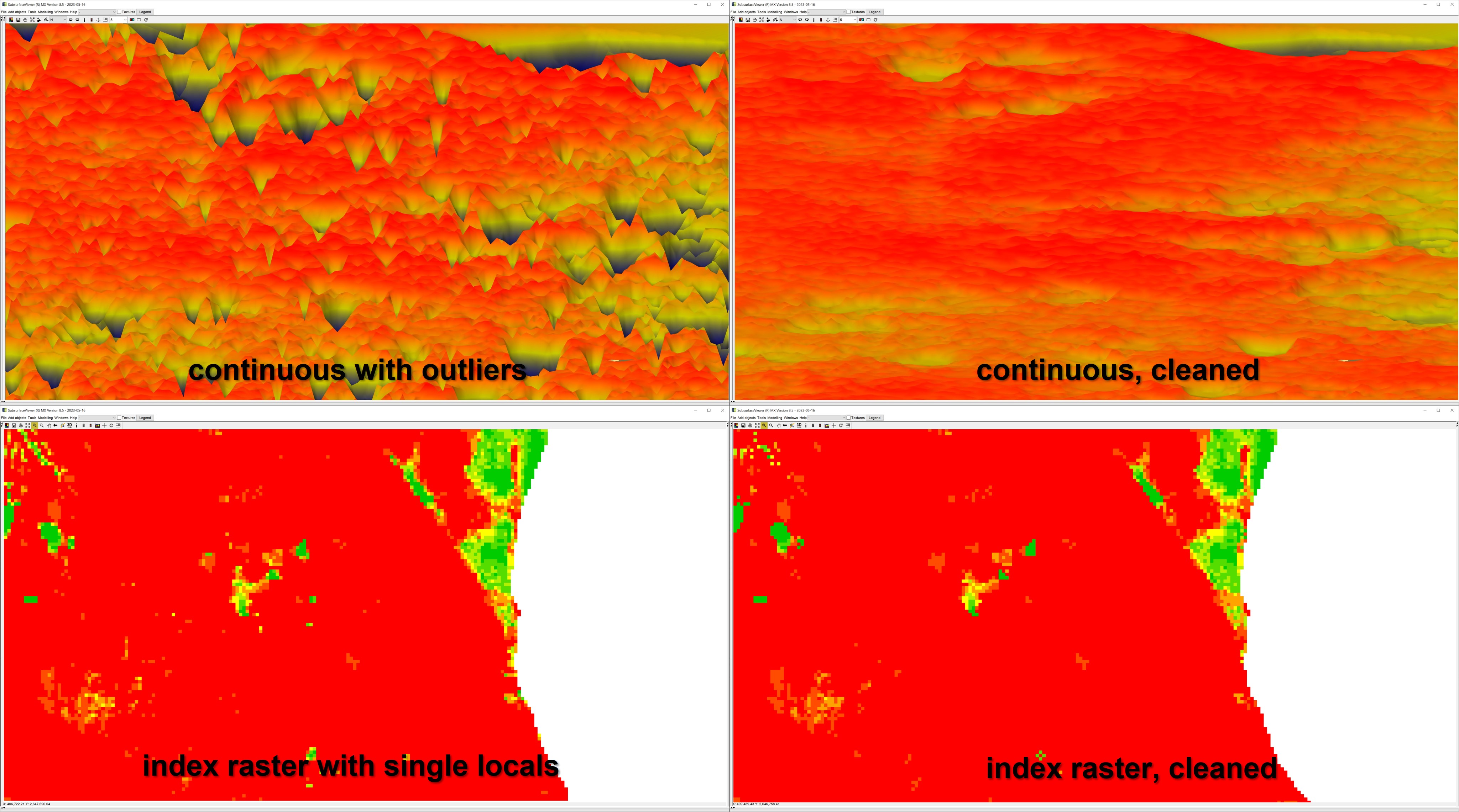
Below are two examples of a clean-up (continuous data and index grid).
Note:
We experienced that better results are achieved with larger search field windows. The calculation takes more time, but the result is more plausible grid values.
¶ Add raster statistics to polygon-shape
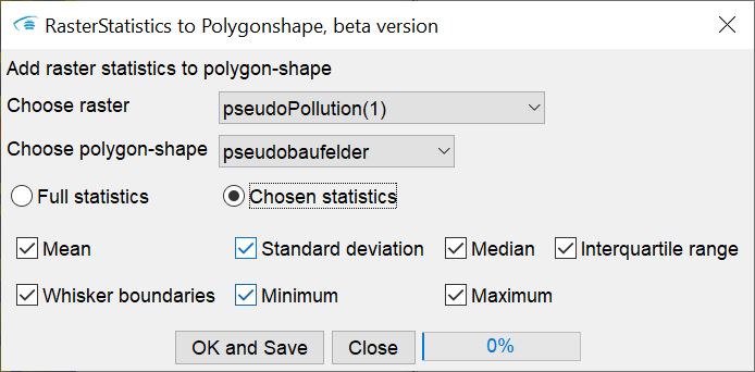
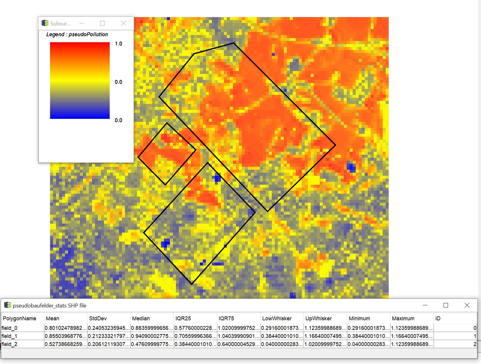
With this function you can write parameters of the descriptive statistics of a raster into a polygon shape (ESRI *.shp) and export it as a new file. Statistics are created for all raster cells that lie within a polygon and assigned to this polygon accordingly.
A typical application would be to transfer a suitability map in raster format into a polygon-based suitability map. Another application could be for the calculation of excavation costs in the case of remediation, for example. If the pollutant is available in a raster format and the excavation plan as polygons of the construction fields with their target depths, then the mean values, median values and other parameters of the pollutant distribution could be assigned to the corresponding construction field here and passed on to the application. See an example below:
¶ Convert XYZ Table to raster
You can write XYZ files in the SubsurfaceViewer via a small function into a raster without a concrete interpolation. This application may be needed, for example, when rasterised XYZ files are supplied for elevation data. A good example are the freely available ATKIS® digital terrain models (https://www.adv-online.de/AdV-Produkte/Geotopographie/Digitale-Gelaendemodelle/). The tile datasets can be loaded individually or in a batch. Grid cells for which no height coordinate can be found are assigned a NoData value.
Note:
If you set the files with a coarser resolution than the original dataset, mean values are formed for all height coordinates that fall within a raster cell. This is a simplified solution. For DTM data in the regional case and a regular coarsening, without the cells overlapping to different degrees, this method will probably suffice. Otherwise, we recommend triangulating on the XYZ data and exporting rasters with a different resolution. For more information, read the article Triangulation. Alternatively we recommend the free SAGA-Tool Resampling. Here you have some additional settings for a raster conversion to other resolutions.
XYZ files are also supplied from geophysical surveys as part of the provision of prominent horizons. In some cases it is not advantageous to perform an interpolation on these data, so you can deal with the data in a similar way here.
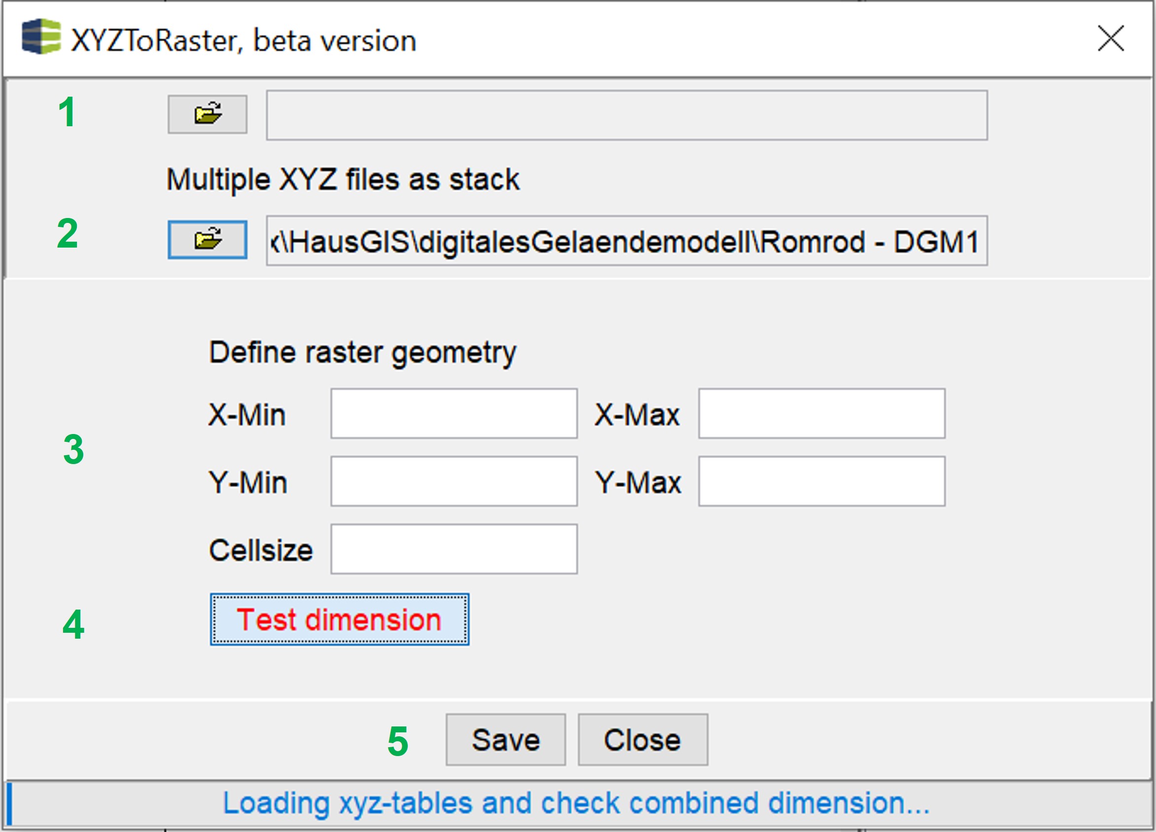
- Load a single XYZ file to process.
- Open a folder from which all XYZ files have been selected (subfolders included).
- Here you can define the extension and resolution of the output raster. When loading a file, a suggestion will be shown.
- If you use file stacks, the dimension of the input file(s) is not checked immediately for time reasons and entered as the default option for 3. To make up for this, you can use this button (not necessary if only editing one file or output dimension is already decided). Enter the correct values in the text fields provided (3.) and start your calculation.
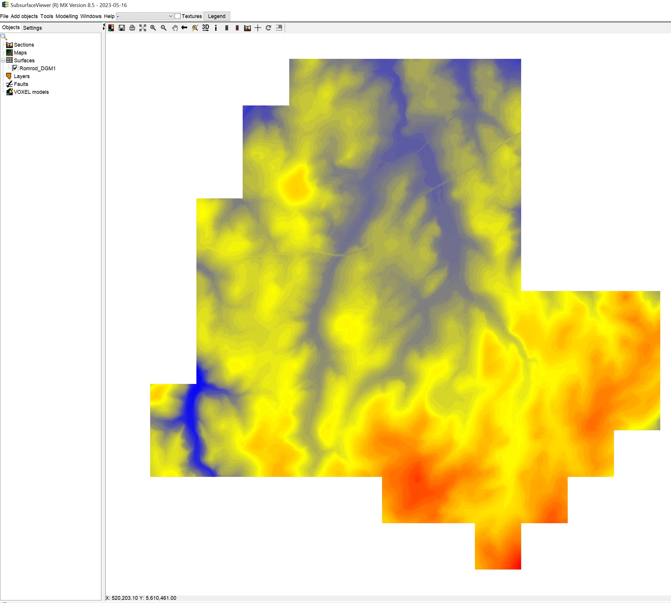
Here you can see an example of a generated raster from ATKIS®-DGM1 data: Sourece
Note:
Note that depending on the resolution, number and size of the XYZ file(s), the creation of the grid may take some time. It is advisable not to make this calculation in the project currently being edited, but to open a new SubsurfaceViewer window for this purpose.