Here you will learn the possibilities of carrying out classifications in SubsurfaceViewer in various ways.
¶ Lithological classification
You can classify lithological data in SubsurfaceViewer using functions of the parameter manager.
The lithological data should either be available in the form of sieve grain analyses or have been derived as similar equivalents from layer descriptions. You may also want to use our parser for layer descriptions. We would like to develop the parser further, so feel free to contact us if you are interested.
¶ Manually
You can classify your lithological data manually in the soil type module of the Parameter Manager.
To do this, follow the instructions in the linked article on the soil type module.
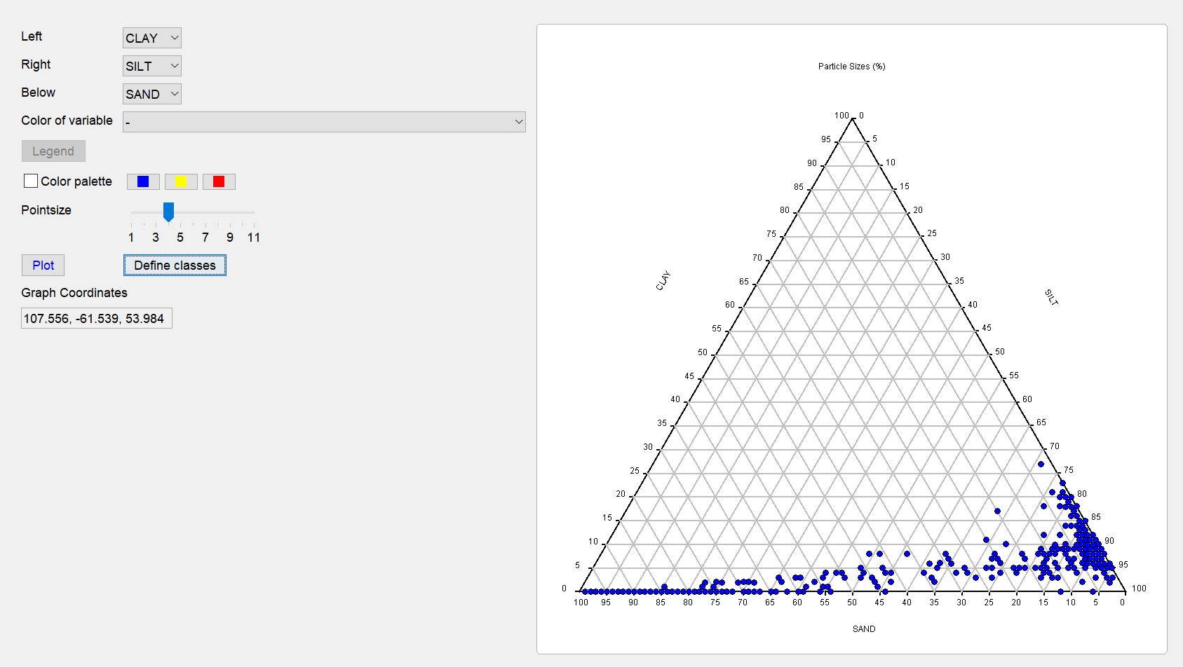
Once you have created a first ternary diagram of the grain size distributions in the sediment, you can start classifying. To do this, open the window with the ternary diagram via the button define classes.
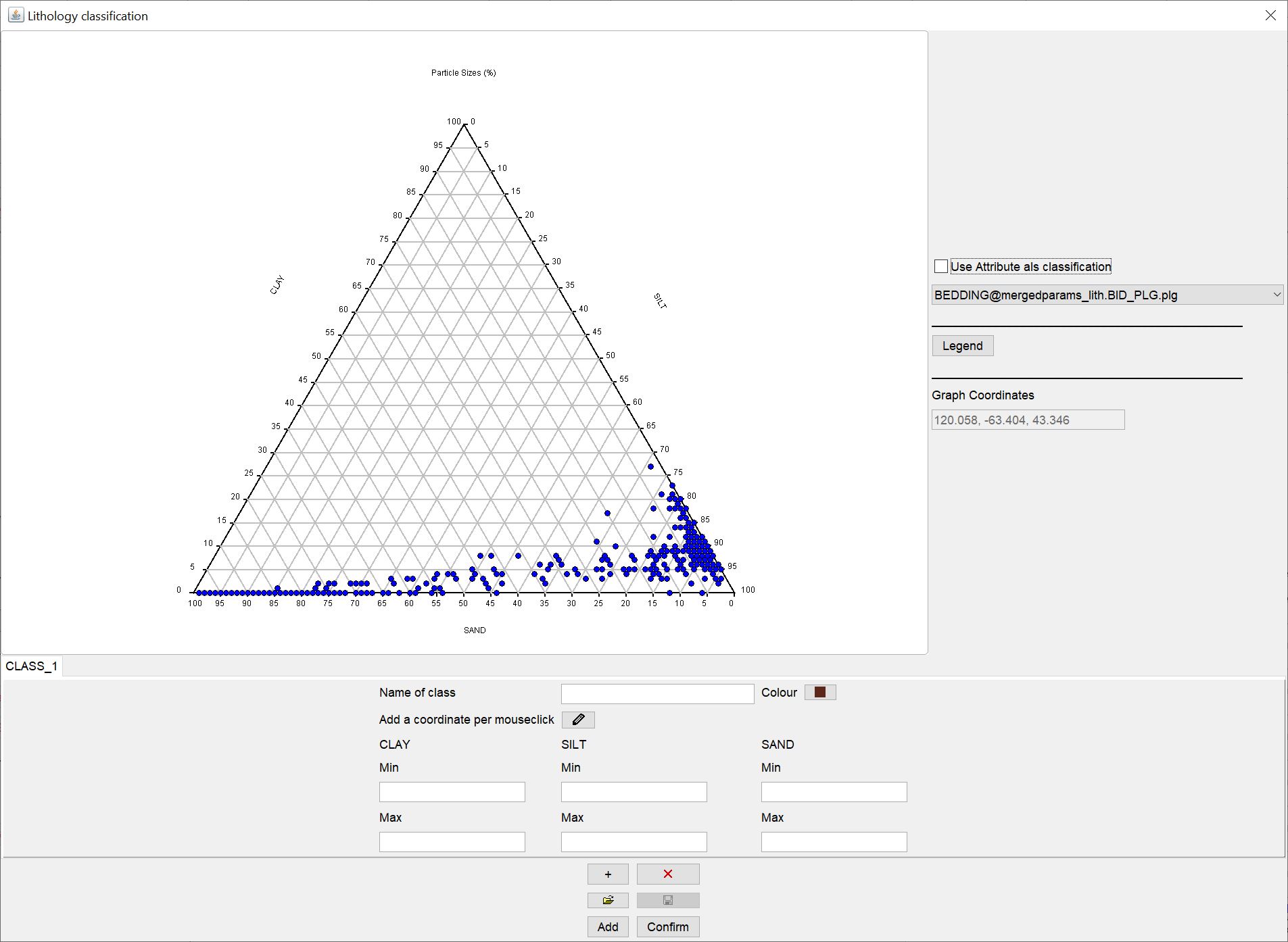
In the new window you will see centrally again the ternary diagram over the grain sizes you have selected and the corresponding axis settings.
On the right-hand side, you can also select an attribute from the dropdown list in a simplified way, if required, to define the lithological classification. The attributes would have to sit at the same coordinates of the lithological samples to be assigned correctly. This option is the simplest and least interesting way of classifying, but can come in for easier use of the HCE module.
Further down you will see a larger options field with which you can manually define lithological classes.
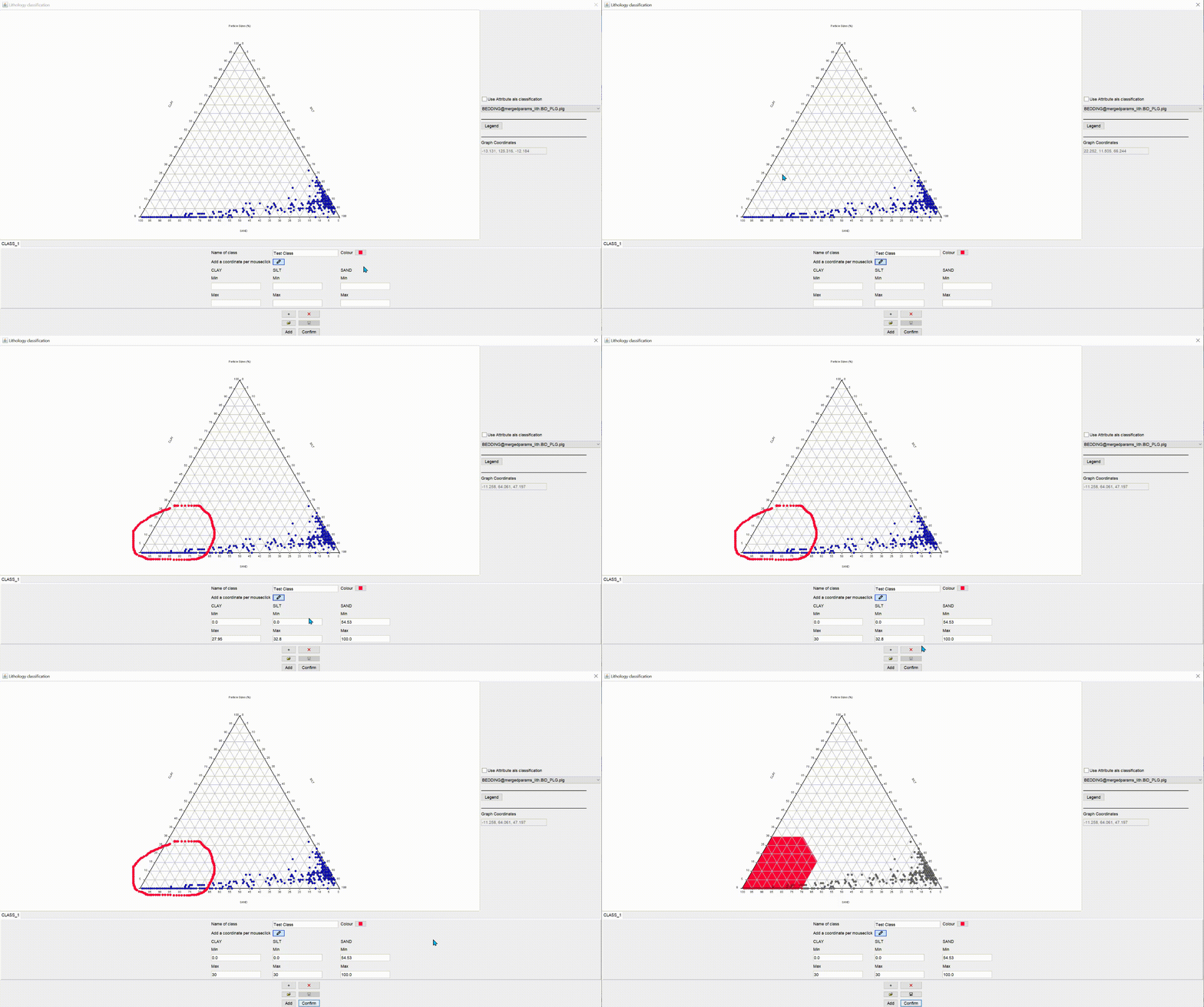
You enter a name for the first class under name of class. With colour you define the colour of the class. In the text fields below, depending on the setting of your axes in the ternary diagram, you can directly enter the min-max limits for the percentage content of a grain size in the sediment for this class. If you prefer an interactive version, you can also press the button with the symbol  . You outline the field in the ternary diagram that matches the target class by holding down the mouse button. You can also click on the corner points. In the text fields you can adjust the values to your needs. If you double-click with the active
  symbol in the ternary diagram, you delete all values for the class and can start from the beginning. With the inactive
  symbol, double-clicking causes a pop-up window to open inviting you to save the ternary diagram to an SVG image file.
If you want to see an provisional result of your classification, press confirm. If you press add, this classification will be added to an already existing one. This is useful if you change the axes of your ternary diagram, open this window again and add more classes that include other grain size fractions.
To add another class, use the button with a + symbol at the bottom. The button with the red X next to it deletes the class currently in the foreground. If a class is added, a new tab appears immediately in which you proceed in the same way as with the first class. There is no limit on defining classes.
The  symbol is inactive until you have pressed the confirm button. Then the classes are in the system and can be saved. They are written into a *.LITHXML-file developed for this tool. You can also reload this file with
  , that you may only have to do an elaborate lithological classification once manually.
Note: If you have used the add option in several different ternary diagrams, each with different axis settings for the grain sizes, the saved LITHXML file will contain all the classes you have entered. If you load this file, only those classes will be visible (after confirm) that match the axes of the currently visible ternary diagram.
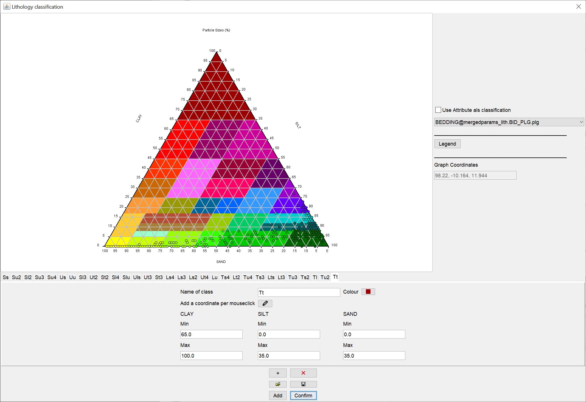
Here you can see an example of a complete lithological classification.
¶ Automatic
We have gained some experience with automatic clustering procedures for lithological data. You could try our implemented Python interface for clustering.
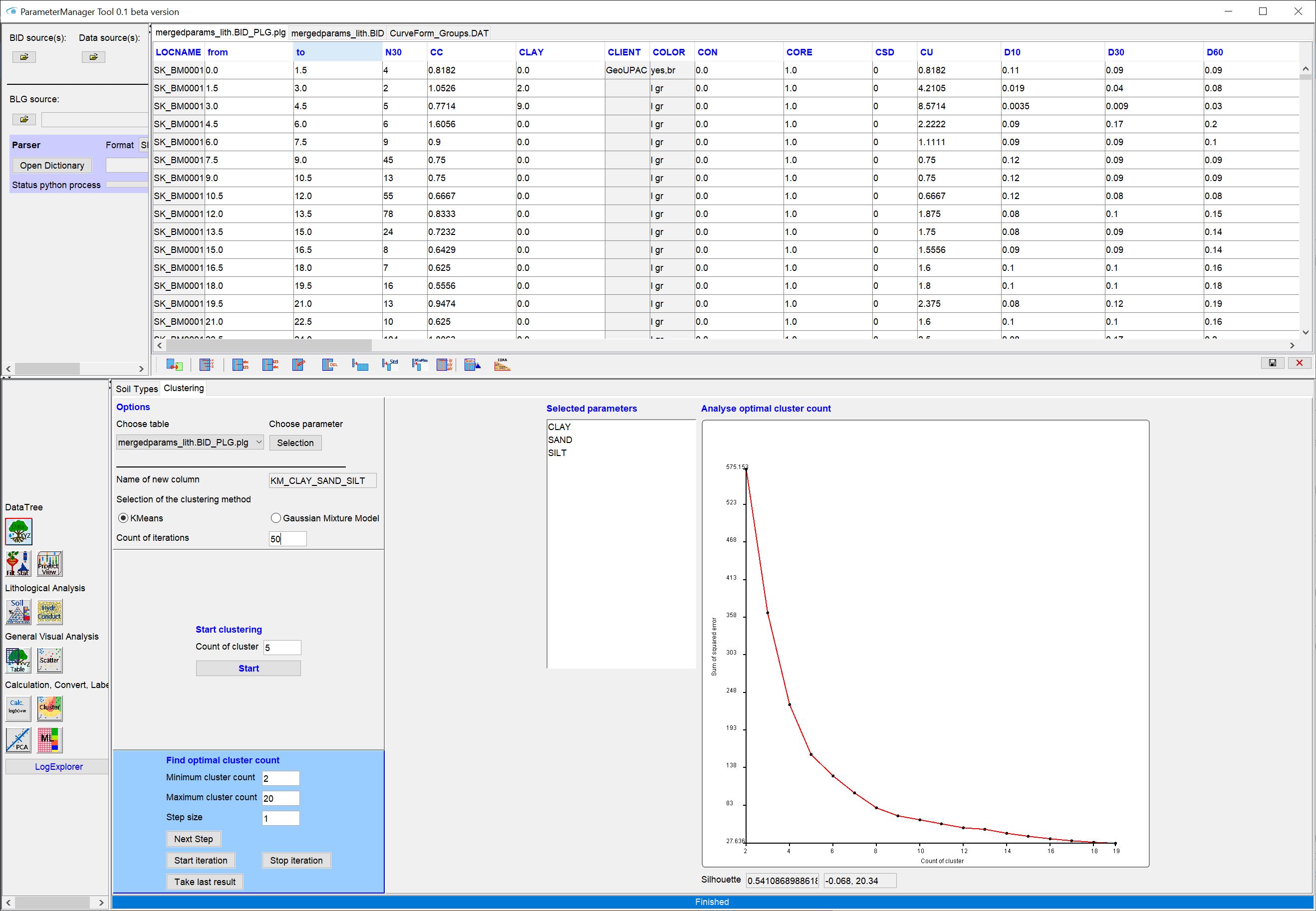
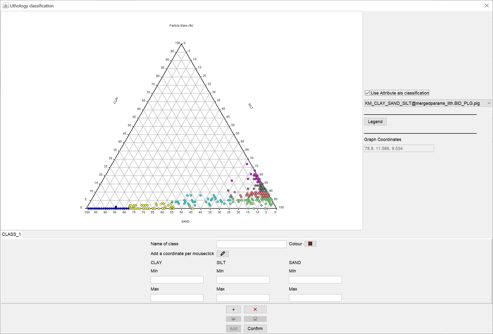
This is especially useful if you are still undecided about the advantages and disadvantages of certain lithological classifications in the area.
In the example we have used K-means clustering, which in our experience works very robustly, as it is essentially based on distances of the value points to each other. More difficult is the use of the Gaussian Mixture Model. Here you may have to perform log-ratio transformations on your grain size percentages beforehand. You can do this via the toolbar for tables in the Parameter Manager.
Share your experiences with us if you like. We are curious to know which methods are most beneficial to you in practice. Just write us an email or give us a call.
¶ Classification of parameters
Use our implemented Python interface for clustering to automatically classify certain parameters.
For classifications that should include a spatial reference, you may use a combination of filtering and editing a new table. We have not tried this yet. But have a look at the articles under parameter manager, logexplorer and LocView-Object. Maybe you will find a creative way through this.
¶ Classification of raster and voxel data
Raster and VoxelData can be classified by a combination of the filter and the calculator for rasters or the Calculator for Voxelmodels manually.
Note: Geofactors already provide possibilities for classification with their Settings. Read the descriptions for the evaluation of a geofactor.
Since the manual classification of raster and voxel data is the same, we will show you the procedure for a voxel model below. In the example we have used the voxel model from the 3D-NORG-project of the Hessian State Office for Nature, Environment and Geology (HLNUG).
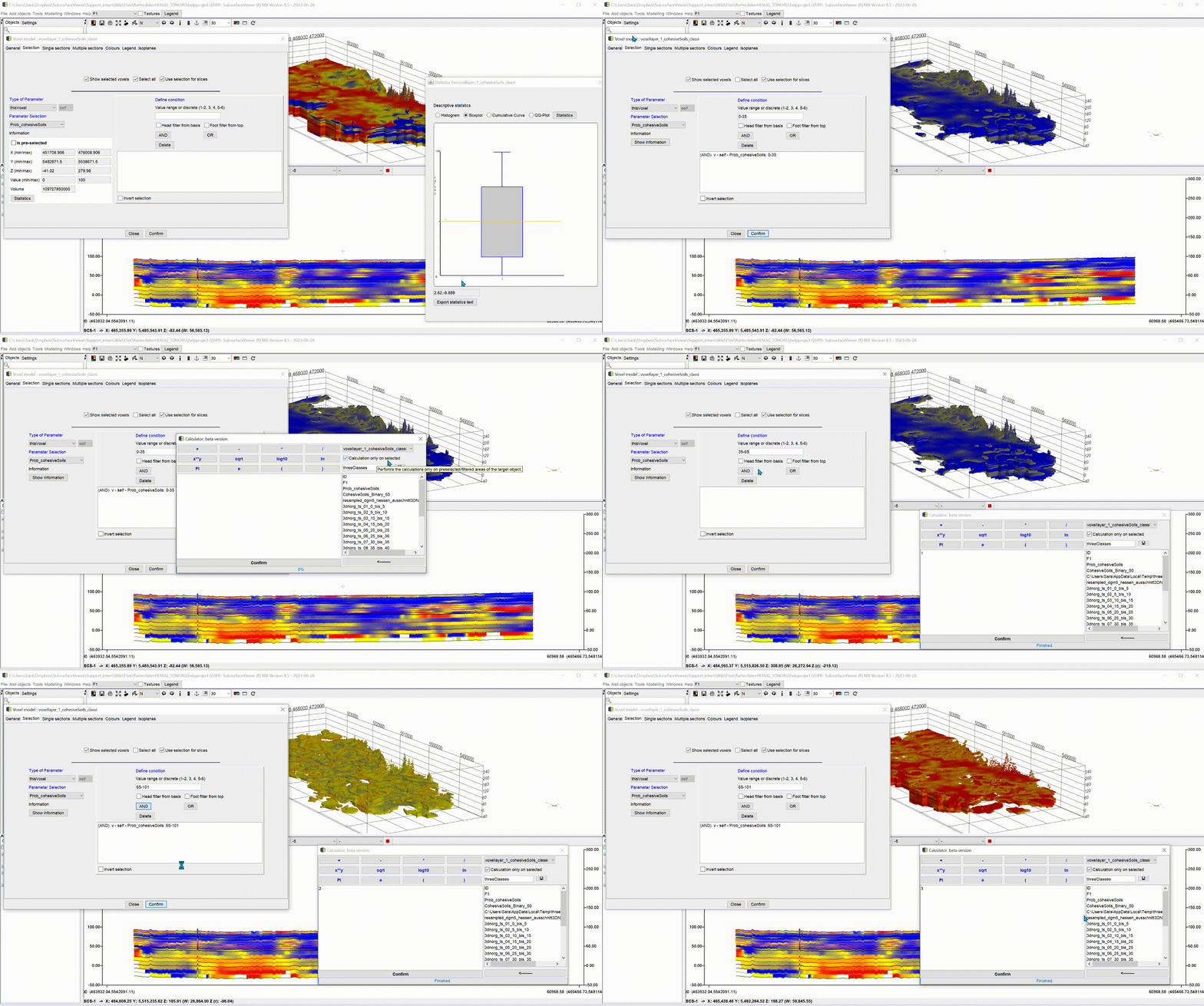
We have a range of values between 0 and 100 in the column "Prob_cohesiveSoils". 0 means that cohesive sediments are not likely to be present. 100 indicates a 100 percent probability of the occurrence of cohesive sediments. There are three classes for the occurence probabilities:
- 0 - 35%, very low probability of the presence of cohesive sediments,
- 35 - 65%, the presence of cohesive sediments is possible but not certain,
- 65 - 100% (101 because of float number precision), a presence of cohesive sediments is very likely.
- Open the filter via the Settings of the voxel model and select those voxels that encompass the value range of the 1st class.
- Then open the calculator for voxel models. Set a name for the classification in the small text box at the top. Leave the check mark at Calculation on selected active.
- Enter the number 1 in the formula window and confirm. The calculator window must remain open and the name of the classification must not be changed.
- Select in the settings of the voxel model with the filter the voxels that contain the value range of the second class. In the calculator window we enter a 2 and confirm.
- Repeat the same for the 3rd class.
- Save the voxel model and append the new column of the classification if necessary. Close the calculator.
Below you can see the result:
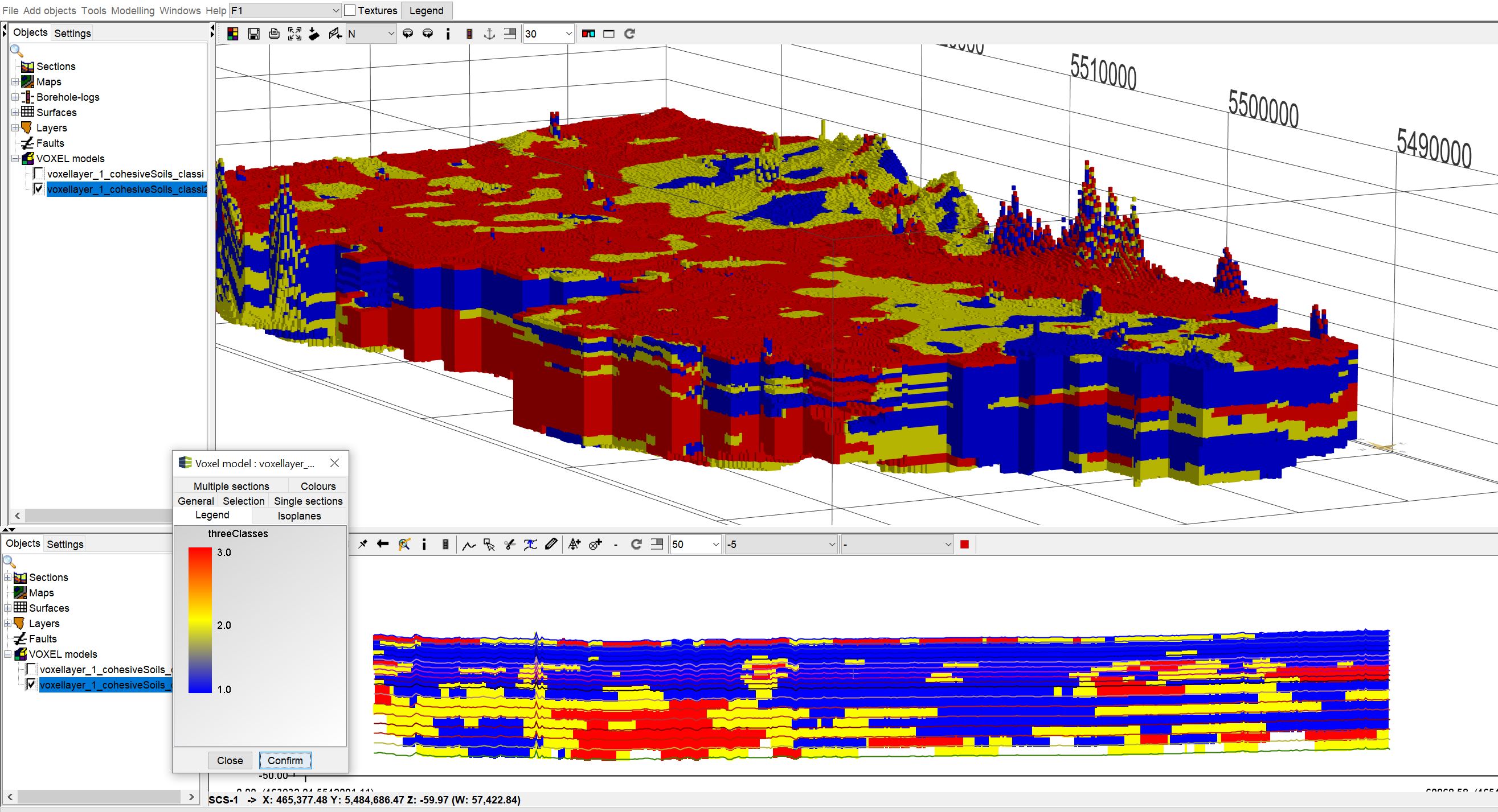
Note: The calculator uses the temporary directory to store the intermediate results. These are not allowed to be deleted during the calculation period. There need to be enough storage space in the temporary directory. This can be relevant for large voxel models. You can select the temporary directory individually via the programme settings.
¶ Layer labelling
By layer labelling we mean the setting of labels on spatially set parameters or layer descriptions. The label designates a geological layer, such as a lithostratigraphic unit. Depending on the processing status, there are different options in SubsurfaceViewer.
¶ Classic option
For this you can use the profile section constructions(/en/HowTo/Profile Sections) to plausibly correlate layers at boreholes with each other.
If you have already created a geological layer model in this way, you can also load the files that you have loaded in the classical style via the boreholes into the parameter manager.
Export synthethic logs from the layer model at all XY positions of the *.bid with the function export layers at BID positions.
You load the table in the parameter manager to the other tables. Use table extraction, and select an attribute from the *.blg file, which is certainly entered everywhere, for example petrography, as the primary parameter.

The extracted table shows the strata data of the boreholes with the labels of the created geological strata model.
You can also load this table into the Parameter Manager and use the tools for evaluating table contents there, e.g. the occurrence of certain terms in pairs. This gives you the opportunity to check your model for plausibility using the borehole information and to verify it if necessary. It is especially relevant if you have a large number of boreholes (>1000) in your conceptually created model as basic information and you could not include all of them in your profile sections.
If you do not want to extract a table, but look at the layer labelling together with downhole curves (for example LITH_COARSENESS (the lithological coarseness curve)) in the LogExplorer and adjust it with the unit functions there, you have to load the table you exported with the function export layers at BID positions into the parameter manager and update the Data tree. Then follow the instructions you find in the linked article on LogExplorer.
Alternatively, you can use the contents of a regular voxel model with layer IDs for labelling in the same way. Use the function Extraction at XY from voxel model.
¶ Experimental extended classical option
Follow the classical way and create an extracted table with the shift labels at your borehole information.
Use this table with the built-in shallow machine learner functions in the parameter manager. Use the shift label as a training label. If you have boreholes available that have not yet been labelled, add them to this table.
The Python tools we have included can derive rules of thumb for layer labelling from your conceptual idea and make them visible, given enough features. If these rules of thumb cannot be recognised again, seem implausible, or the estimated labelling is significantly different from that of the model, you can get to the bottom of the causes. The data basis of your conceptual model may allow very flexible interpretations and these may not have been followed consistently.
Prepare the attributes that you have sighted most to correlate your strata (e.g. sediment colour, lithology, etc.) in your spreadsheet so that they can be used as numerical features by the machine. Use the toolbar for tables for this.
Start the training process with the shift labels and the selected attributes and select the setting all vs all.
You will get an extended table with the estimated labels of the machine that lead to the best solution based on the training on your attributes. You can compare the result with your labelling and look at the feature weights (feature importance).
Are the results plausible? Where are stronger discrepancies? Why? Why don't you load this table into the data tree and create LocView-Objects with the labels and the estimates. Can you use this to verify your model more quickly? Why yes or why no?
If a layer has not been estimated correctly several times, you can approach the labelling with the setting one vs rest. To do this, follow the instructions in the parameter manager. Ask the same questions as above and evaluate the results.
If you have a dataset of layer descriptions that have already been partially labelled with layer assignments, and you are at the beginning of modelling, you can use the corresponding label training to label still unlabelled boreholes. Use LocView objects for visualisation in your profile sections or in the 2D/3D view. This could be a good aid for you to get an overview of the data and to be able to type first characteristics for certain layers.
Note: The described process is to be understood as a suggestion to first approach the usefulness of machine learning methods. The tools and ways described are initially intended to get you started and to support your modelling in pre- or post-processing. You should always view and check the results carefully. Do not immediately use them to quantify uncertainties. That would require more! You should test different settings and combinations of characteristics. If you want to go deeper into the topic, you should work directly on the available Python libraries.
Feel free to contact us if you are looking for more intercommunion
Please note that some of the functions in the parameter manager are still in a beta state because we have not had the opportunity to test them. So please get in touch if you find something that seems like an error.
¶ Flexible manual labelling with LogExplorer
In order to use the labelling functions in LogExplorer, you must have the layer information, i.e. corresponding characteristics, available in numerical form (downhole).
If you "only" have access to layer descriptions, you could look into the parser for layer descriptions and the lithological curves. We would like to develop the parser further, so feel free to contact us if you are interested. You can translate your layer description content into numerical values in other ways. In the end, we only need ASCII tables with a suitable separator. If necessary, read the article on formats.
In any case, the corresponding tables containing the data must be loaded with the parameter manager. Follow the instructions in the linked article. Do not forget to create the data tree. Then open the logexplorer and select one or more features to illustrate with downhole curves. If you have core photographs, have a look at the Core Texture Tables article. Because you can load them as background images to your curves. Then follow the descriptions you see LogExplorer in the section labelling -> units. Use the data tree and the LocView-object to see the generated layer labels in the Profile Section or in the 3D-View and check them for plausibility.