This section explains the inverse distance weighting tool for interpolating data in 2D and 3D. You will find these functions in the main menu bar under modelling. For the format of the input data, please read here.
If you want to know more about the calculation, we recommend the Wikipedia explanation: https://en.wikipedia.org/wiki/Inverse_distance_weighting.
Summing up inverse distance weighting calculates a weighted average of the input values at the interpolation point, normalised to the sum of all weights. The weight, i.e. the influence of an individual input value on the mean value at the interpolation point, is measured by its distance from the interpolation point - strictly speaking, by the reciprocal distance with an exponent specified by the user. By increasing or decreasing the exponent (power of weighting), the user controls whether the influence of a point decreases more or less rapidly with distance. The formula for weight calculation from Wikipedia is included here for better understanding:

wi = weight of an input value i.
x = location of the interpolation point.
xi = location of the input value i.
d(x, xi) = distance between interpolation point and input value i.
p = exponent set by the user.
The formula above illustrates that a high value for the exponent means that an input value loses its influence at shorter distances because its weight becomes very small.
Here is the complete calculation of the interpolation point:

u = result at the interpolation point.
ui = value of input.
The formula above shows that at an interpolation point that lies at a very short distance (~0) from the input value i, the input value i is set and all other points no longer have any influence.
Besides the definition of the exponent, you influence the calculation by an input in the section max.point number, which can be found in the 2D- as well as in the 3D-IDW tool. If an interpolation point is calculated, all distances to the input values are calculated and then sorted by distance in ascending order. If you do not use the entire number of points (input value = 0), only the input values that are closest are used for interpolation. For example, if you enter 10, only the 10 closest points from the interpolation point will be included in the calculation, all others will be ignored. You should take a closer look at the spatial distribution of your data to prevent the creation of implausible results. This is important if you have spatially structured data with a strong uneven spatial distribution. Limiting the number of points can be useful if you go in with a data set >~5000 points. Then the calculation can take longer and you could reduce calculation steps with this.
Voronoi mit IDW erzeugen:
If you internalise the calculation procedure described above, you can use inverse distance weighting to perform a Voronoi decomposition of the area.
This is written in 2D or 3D raster formats using this tool. To do this, set the number of points to be used (max. point number) to 1. Then, for each interpolation point, the closest input value for the interpolation point is ever used, which means that no more averaging takes place, as the weight of this point normalised to itself is always 1. This automatically results in a Voronoi decomposition. If you are not familiar with the term Voronoi, read https://en.wikipedia.org/wiki/Voronoi_diagram.
¶ Inverse Distance Weighting IDW
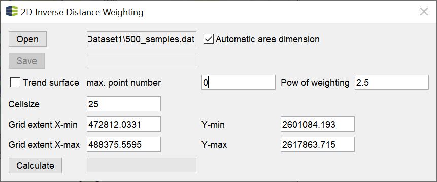
Under this title the interpolation method for 2D space can be found in the menu modelling.
The handling is kept very simple. Open your data with open (formats). As soon as you have loaded them and the check mark at automatic area dimension is active, the text fields for the dimension of an output grid will be suggested immediately. If you want to know which output formats you can expect from this function, you can look up the formats for raster data here.
Read the introduction of this article to understand the text fields max. point number and pow of weighting and to enter meaningful values. By default, max. point number is set to 0, which means that all input values flow into the calculation of an interpolation point. Pow of weighting suggests a value of 2.5 by default. We recommend calculating several calculations with variations of the exponent and evaluating the results for plausibility.
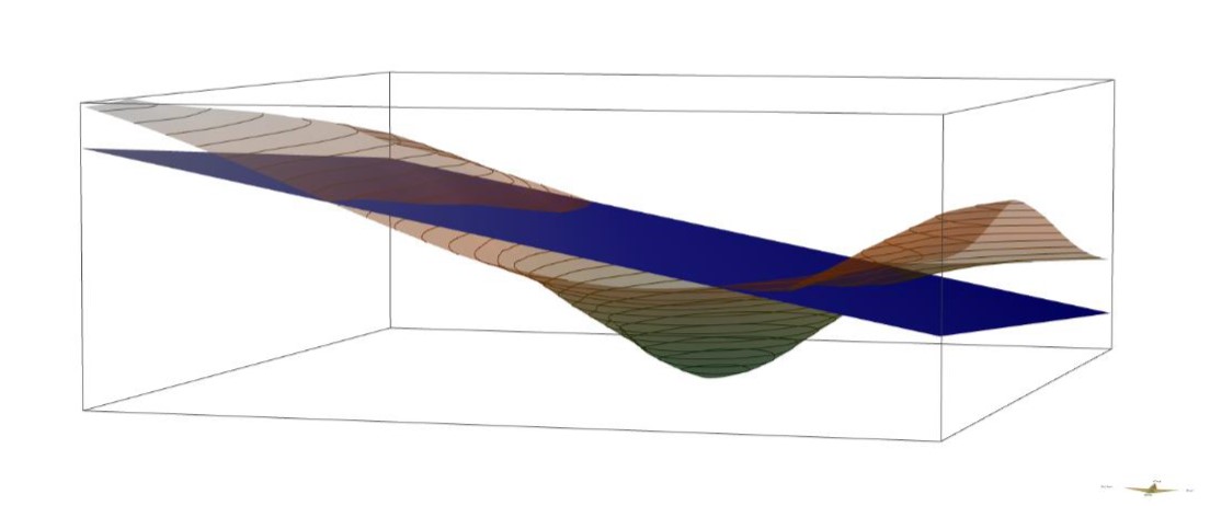
If you tick trend surface, a linear regression is calculated over the input values before the interpolation. This creates a linear trend surface. Then the residuals, i.e. the deviations of the input values from the trend surface, are calculated. The residuals are used for the interpolation calculation. Once this is complete, the interpolation value is calculated back from the trend surface. This way you get an interpolation that is not distorted by a global trend. If there is no trend at all in the area, the result will differ very little from one where you have not set a trend area calculation. Keep in mind, that if you have a lot of input values, the regression will take some calculation time.
Note:
You can also look at the calculation protocol in the info-window. There you will find the parameters of the trend area calculation. At "trend=v1 v2 v3" the three parameters are listed, which you calculate with v1 * x + v2 * y + v3 to get the trend value at a certain location. At "y=..." you see the gradient of the linear trend, where x and y are not to be confused with the XY coordinates. This formula refers to the slope of the surface.
In the examples below the results of different calculations are compared:
¶ With and without Trend
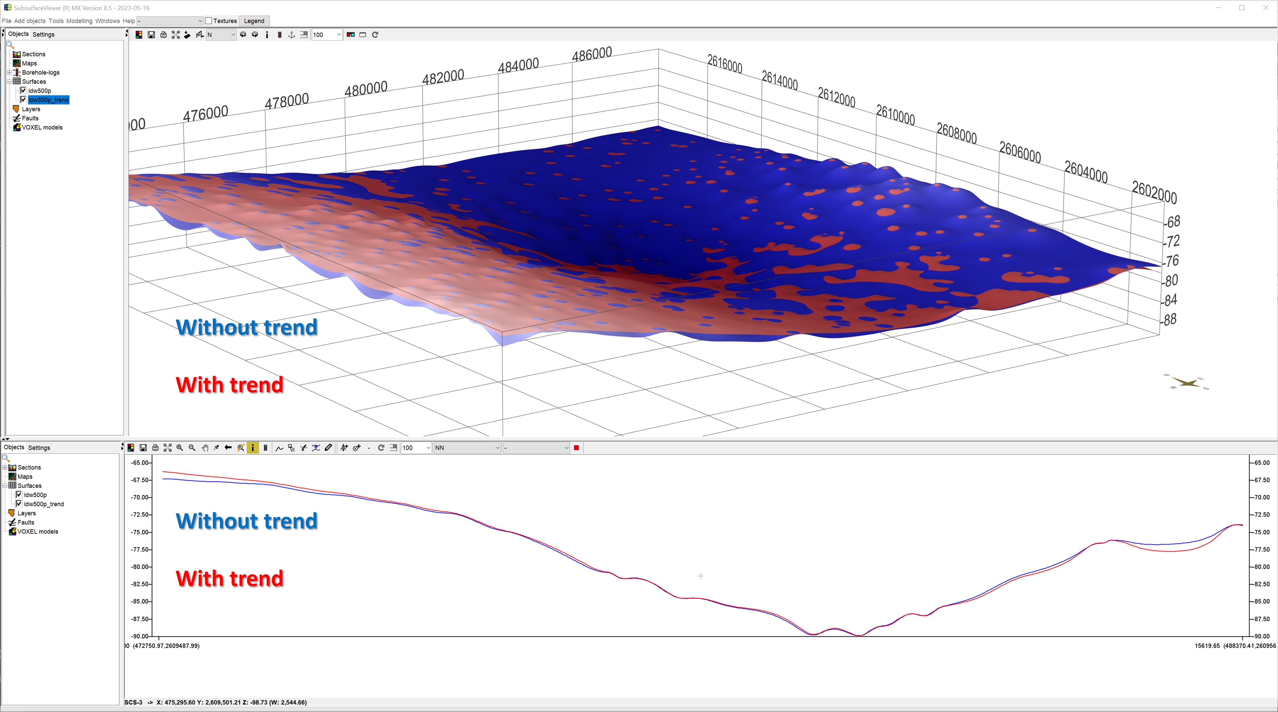
You can see the comparison of an inverse distance interpolation with and without trend area calculation. Since the slope of the trend area corresponds to the example image above, you can see the effect of the detrending before the interpolation on the result.
¶ IDW with different settings
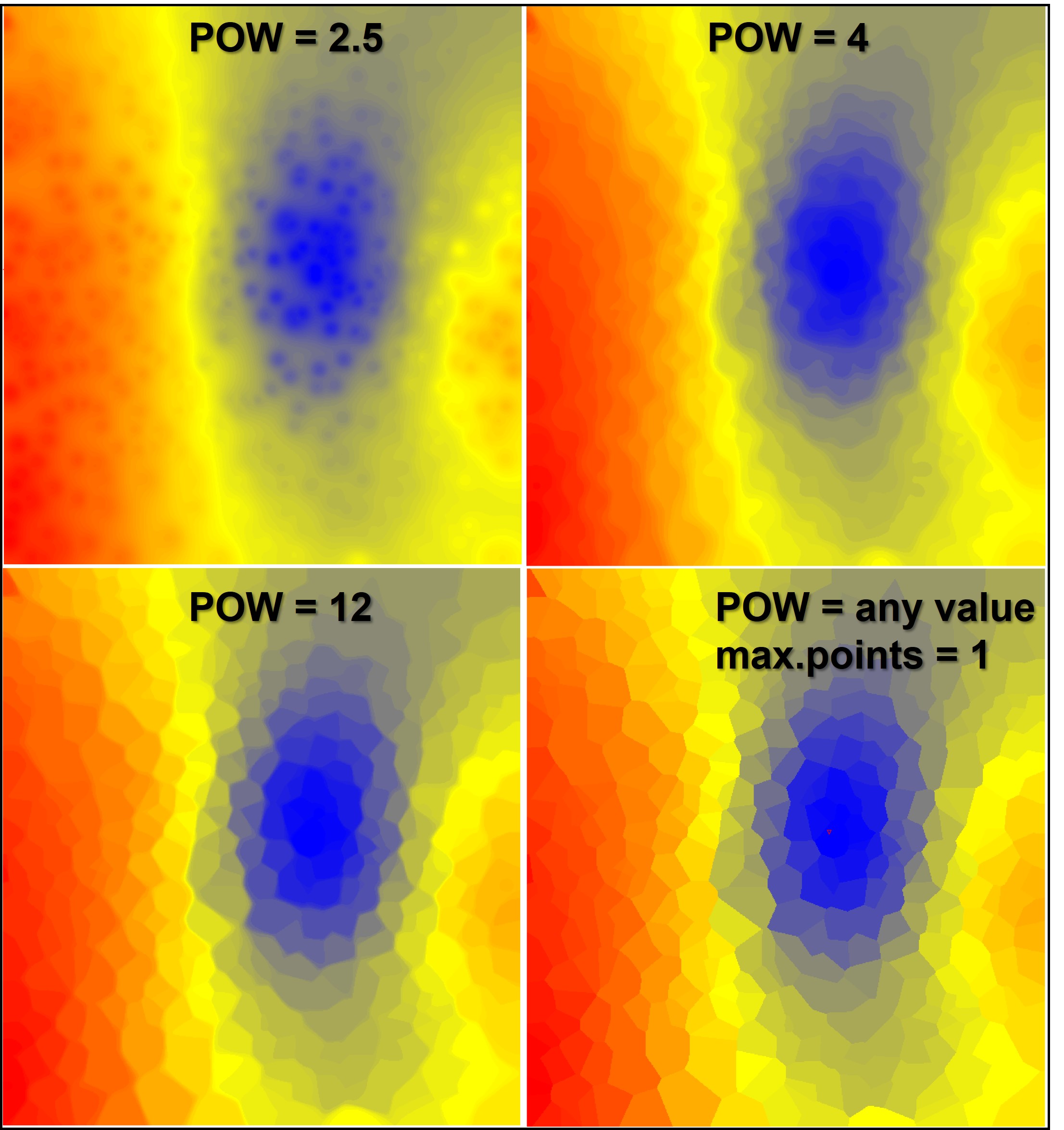
Here is a comparison of IDW interpolations with different exponents. The calculation at the bottom right corresponds to the setting described above for a Voronoi decomposition. You can see from the image below on the left that even a very high exponential value ultimately approaches a Voronoi decomposition, since the influence of values decreases strongly even at small distances. Consider the power rules for negative exponents and smaller than 1.
¶ 3D Inverse Distance Weighting
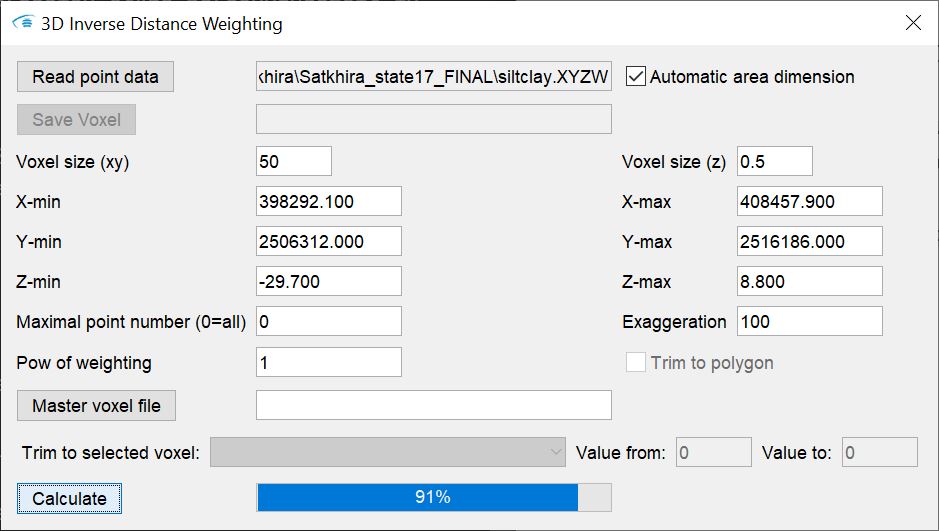
This tool performs inverse distance weighting interpolation in 3D space. The output format is a regular voxel model (formats).
The theory, of course, remains the same as described in the introduction, and the structure of the tool's user interface is similar to that for the 2D-IDW tool.
Load the data in these formats with read point data. Define the dimension of the output in the text fields below. In the field maximum point number (0=all) enter the number of input values to be used for interpolation. In the 2D-IDW this corresponds to the field max. point number. More detailed explanations can be found in the introduction to this page.
For the 3D interpolation you can set an exaggeration factor with exaggeration. This factor represents the vertical-to-horizontal anisotropy common in geological depositional spaces. It significantly influences the distances between points in the vertical and the influence on the interpolation point. In most cases - and especially if you are interpolating data from boreholes - an exaggeration is recommended. Choose a suitable factor by trial and error and checking the plausibility of the result.
The entry pow of weighting corresponds to the exponent you have to choose for the calculation. Read the introduction of this article for an explanation.
If you have stored a polygon in the project, for example an area outline, in the clipboard by copy, the field trim to polygon is active. If you set a check mark here, an interpolation is carried out for voxels within the polygon. All voxels outside the polygon receive a NoData value.
You can also use master voxel file to load a voxel model that already specifies the dimension of the output model and contains other parameters (for example, an IDW interpolation with other settings).
If you want to perform the interpolation on voxels that have a certain range of values for a certain parameter, you can use the options in the trim to selected voxel area. Use the dropdown list to select the parameter on which the condition is to be checked. With the fields value from and value to you specify a range of values as a condition that must be met for the interpolation to take place. You can also perform layer-internal interpolations with this option. You can find detailed instructions on this under layer-internal parameter interpolation.
¶ 3D-IDW with and without superelevation
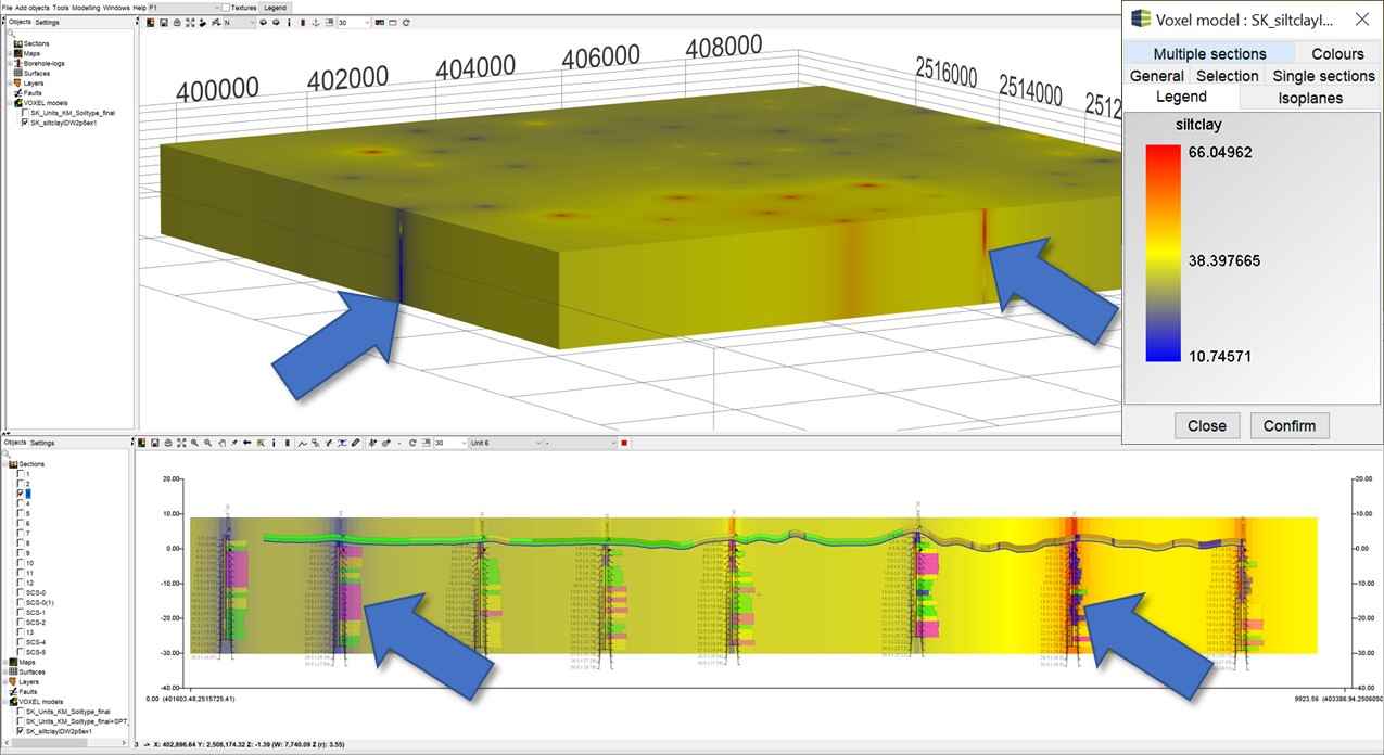
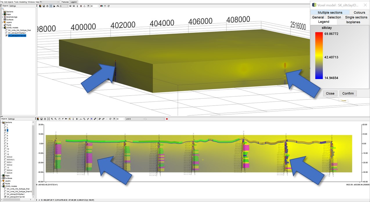
Below comparison of the IDW interpolation with and without superelevation for data from boreholes is shown. The blue arrows help you to recognise striking differences. The data represent the fine grain fraction of sieve analyses from borehole material in the model area Satkhira, which was given by the GSB (Geological Survey Bangladesh) and the BGR (Bundesanstalt für Geologie und Rohstoffe). Note that this is only an example and this form of interpolation is not a sensible way to handle this data.
If no superelevation is set, the data originating from the same borehole will basically be influenced by closer distances to such an extent that data from a borehole further away will be given much lower weights. This means that there is little variation in the vertical of the voxel model, because the boreholes influence the interpolation point "as a whole". With a superelevation, the result looks more plausible.
| Without superelevation | With superelevation (100) |
|---|---|
 |
 |
