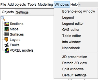
 Under the menu item *windows* you will find various input file editors, such as the legend and GVS editor. Furthermore, the *borehole log* window can be opened here, which appears when you click on a borehole in the 2D-view. The *info window* helps you to keep track of information while working in the project. Further down, under the dividing line, you will find settings for other window arrangements.
 ¶ Borehole-log window
The borehole-log window shows information about the boreholes that have been clicked with the info cursor  . The window opens automatically when you click on a borehole.
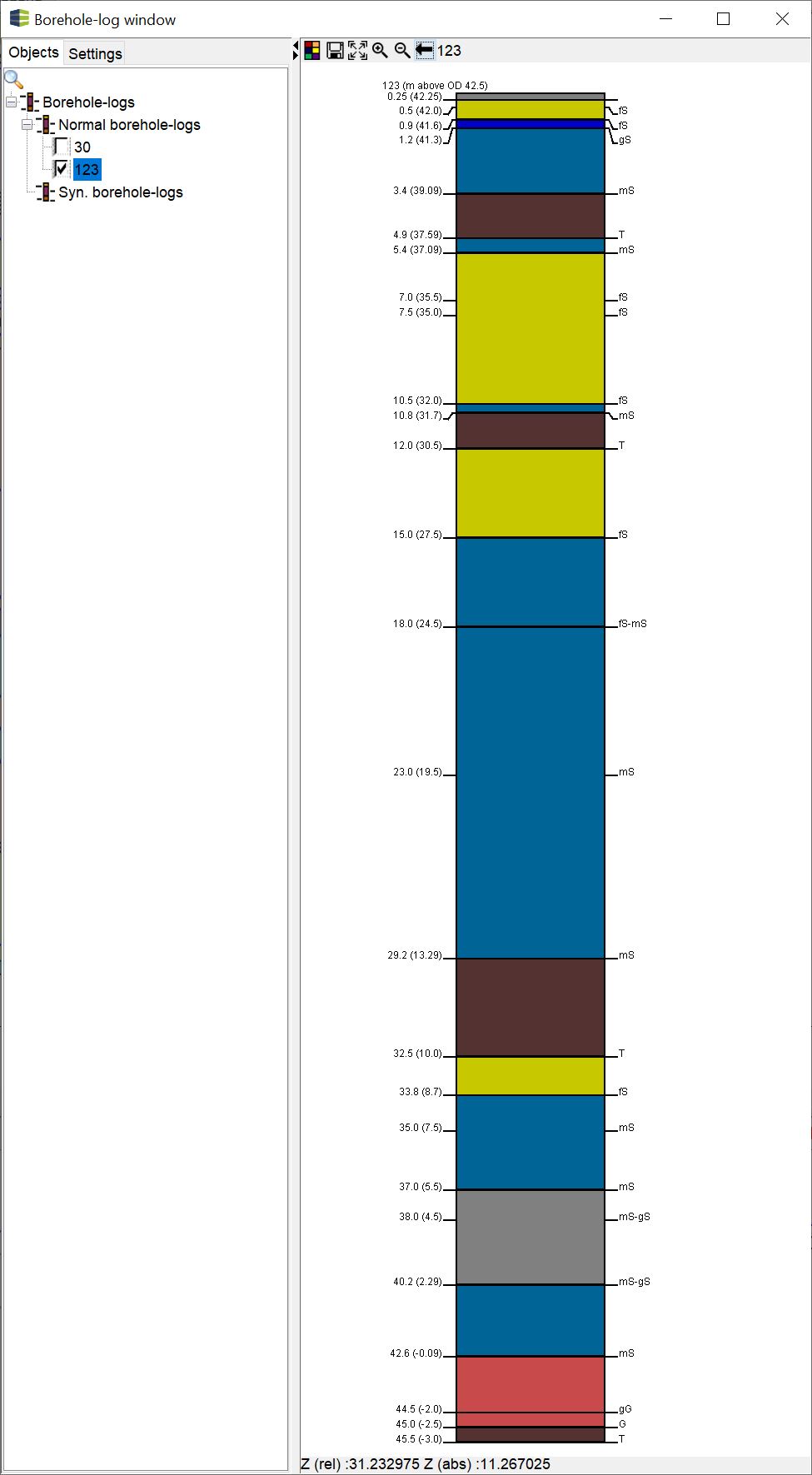
To zoom into the window, you can use your mouse wheel. Otherwise you will also find zoom options in the toolbar at the top. Here you can change the background colour and save the information in the field as text.
The drillings will initially be displayed exactly as set in the settings of the drill point map. You can adjust the settings for these borehole(s) individually by right-clicking on the borehole or log in the object tree to open a menu. With the right-click menu you also have the possibility to display only these drillings in the 3D-View and write a comment or a note. This allows you to manually grade the quality of your holes as you model them, you can accurately incorporate the information they contain into your model.
If you have used the synthetic borehole creation tool, it will appear in the syn. borehole-logs tree.
At the bottom of the window you will see a text field that shows you the relative and absolute depth at the borehole and the respective mouse position.
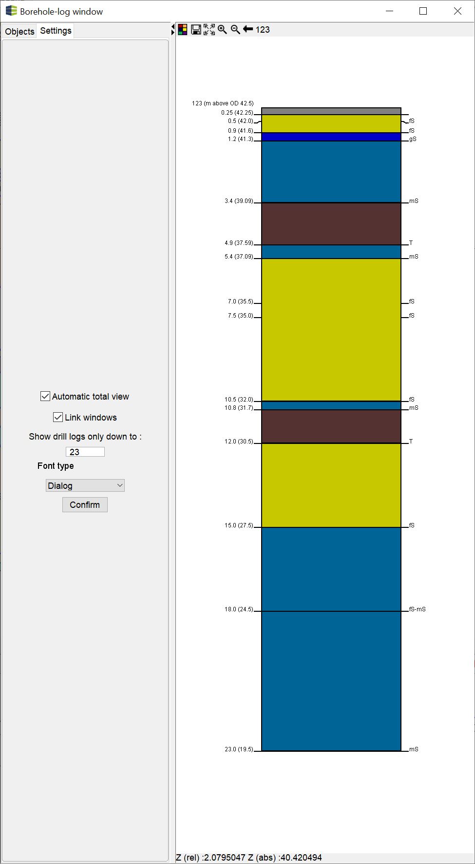
With the settings tab of the borehole-log window you can make more specific settings.
If the check mark automatic total view is activated, the borehole is automatically scaled in this window when you click on the 2D view.
With the check mark link windows, the window is always "clipped" to the left side of the general user interface, if the window was previously closed and an opening was initialised by a click in the 2D-view. If you work with separate windows or with several screens, this can be disadvantageous.
With show drill log only down to you can crop the view to an absolute depth. In the example, the height was limited to 23 metres above sealevel downwards.
With font type you can finally adjust the font for the layer description.
¶ Legend
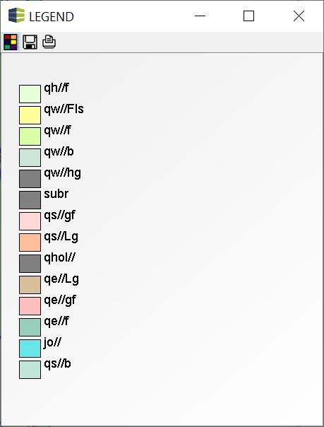
In this window you can see the model legend that you defined in the project settings. You will find the same button in principle in the main menu bar. The same window opens here.

In each case, the part from the legend is shown that is set in the dropdown list of the main menu bar and due to which the modelled layers are currently coloured.
With this tool  the background colour of the window can be changed. With the
  ! tool it will be saved and printed with
  .
.
¶ Legend Editor
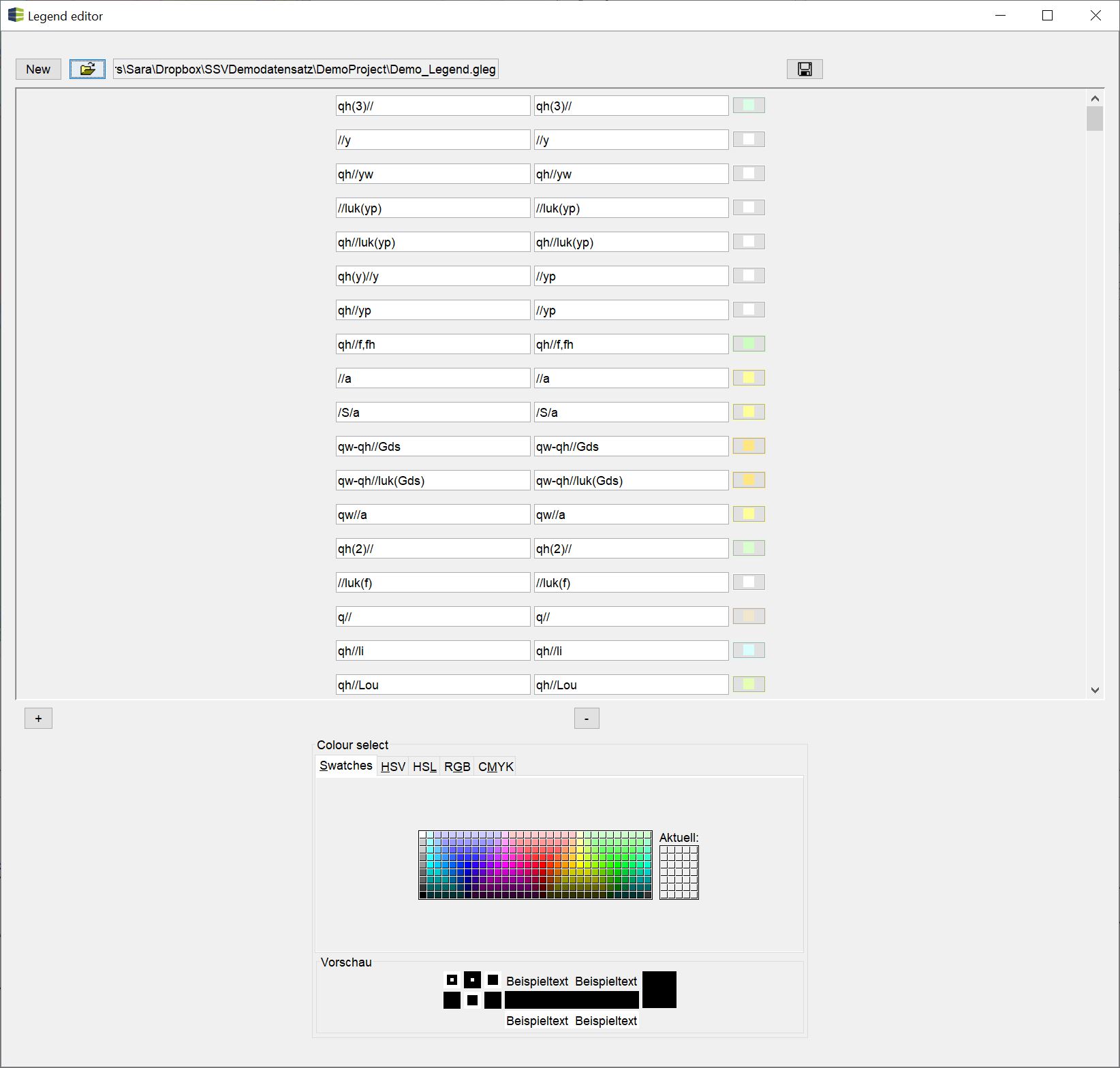
Colour legends are an important part of modelling and evaluation. That is why the creation of a legend is one of the first steps, which schould be done in the project settings. Possible formats for legends and their functions are described here.
An individual legend can be designed in the legend editor. A previously designed table can be opened via  or a new legend created.
With the plus symbol you can create a new entry and select name and colour. With the minus symbol you delete the lowest entry. In the lower part of the window you can see the colour selection. The colour space and colour can be selected here. With the disk symbol  the table is saved.
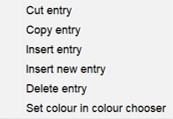
If you right-click in the area of a text field, a small menu opens with which you can insert entries in the correct sort order, delete them or change the selected colour.
Background information:
Save the legends with the following extensions: *.gleg and *.voleg for colourings to be assigned to unique names, such as the name/ID of a geological unit or designated soil type.
Save with the extension *.paleg or *.beleg, there must be numbers in the first legend column. These define the value range for which the colours are assigned. For legends of the type *.beleg, the value ranges greater than or equal to the upper entry and less than the following entry are displayed uniformly with the colour set at the top. This is a value classification via the colour. For legends of the type *.paleg, the value range between the upper and the following colour is interpolated by value.
The second column of the legend allows the assignment of an alias entry if you want to assign a meaning to the value range for a better understanding. We have summarised it here and shown an example.
¶ GVS-editor
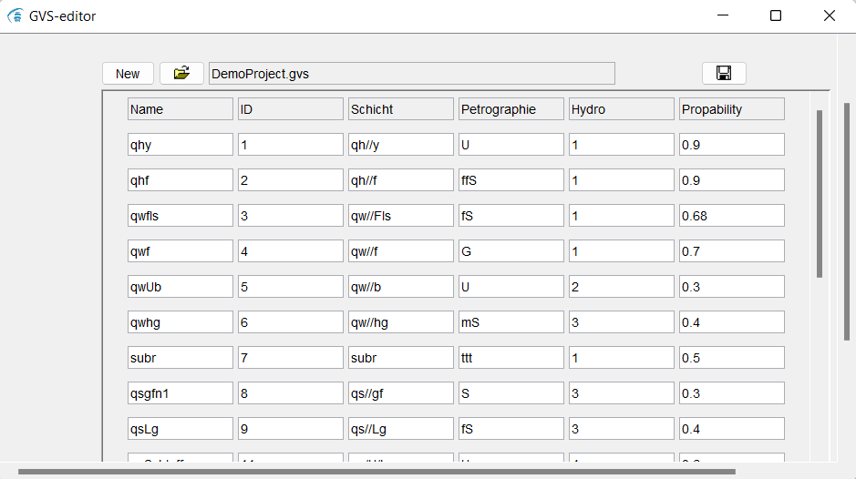
With the GVS Editor you create information that are the fundamental basis for conceptual modelling with SubsurfaceViewer. Without a GVS table you cannot model layers. It is defined centrally and described in the project settings.
In this table you list the abbreviations, names and attributes of the layers in their chronostratigraphic order.
The illustration shows the stored attributes for the opened demo model as an example: the ID, the name of the layer, the petrography, hydro for the identification of the groundwater-relevant layers and probability for e.g. the assignment of a probability with which a certain parameter is defined per layer.
The options for adding and deleting rows are the same in the GVS editor as in the table editor.

The attributes in the optional columns can be selected in the menu bar and displayed for the layers selection of attributes layer description.
Note:
Note the order of your entries! The first column always contains the youngest layer, followed by the older layers or the layers that follow in depth. The ID of the layer must be unique and you should define it in ascending order from top to bottom, according to your position in the table. Generally create a chronostratigraphic list with the GVS table. Lenses are each defined with a layer top and bottom edge, whereby the ID of the top edge is always named with the negative equivalent of the bottom edge, that a clean assignment can take place. Do not mix IDs for lenses with those of the main units.
If you need to adjust the GVS file during your modelling, you should not forget to update it in the project settings.
Note:
If you have already constructed profile sections and subsequently realise that you need to adapt your LSG, you can use the function for renaming the lines under Tools.
¶ Table editor
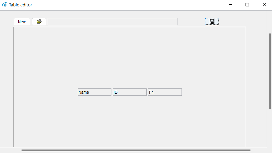
Table notes can be entered in the table editor. Any information can be entered.
Save them with  .
.
With  a line can be added and with
  the lowest line is deleted. In this way you can delete the already existing predefined column titles. With the button
  on the right side another column can be added and named.
With new a new table can be started and with the folder symbol next to it a table can be opened.
¶ Info window
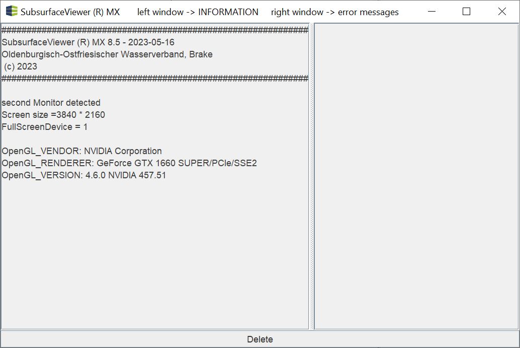
Under windows, the info window can be displayed. Here, information about the programme processes is displayed on the left-hand side and red messages are collected on the right-hand side if errors have occurred. With delete, the information collected can be deleted. In some calculation operations (e.g. from the [parameter manager](/en/Funktionen/Parameter Manager)) or when calling up the info function in the 3D-view, the window is opened automatically to show messages directly. The info window becomes relevant for validating profile cuts via this function. If you are working with kriging, certain calculation parameters are the output for your review.
Sometimes, when you open the info window, you only see the right side and the left side is collapsed. You can slide the bar between the windows and thus open the left side again.
Note:
We recommend that you open this window as soon as you start a calculation. You will receive important information about the programme processes here. You will also have a chance to see an error message if something goes wrong. More information can be found in the section trouble shooting. You are welcome to send us red error messages.
¶ Noticebook
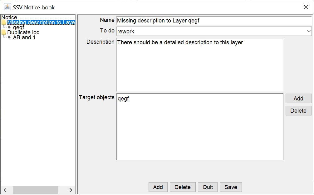
If you want to work on your models with others or document your work, you can use the notebook to make sorted entries.
The name entered for the note at the top determines the category of your note and forms the trunk of your note tree on the left. You can enter a to do note and a description for your category.
To specify the content of the note on objects, add a new target object with add on the right. Another window will open. Under target object select the object category (e.g. boreholes, layer, etc.). A unique entry for identification will help you to find the object in the left object tree. You can enter your detailed note in the description field.
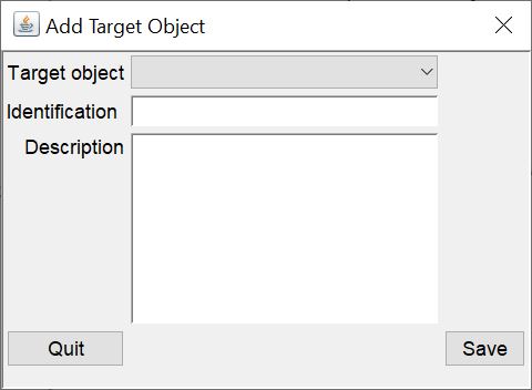
You can add a complete note category with add in the lower part of the window and delete it with delete. However, all your notes on the target objects will be lost.
Note: Do not forget to press save to save your note.
¶ 3D presentation
This function deactivates all views except the 3D view. This setting is used for presentating the model in the 3D view while the model construction is not visible.
¶ Detach 3D view
This function decouples the view 3D-View into a separate window so that it can be moved on a second screen, for example.
¶ Split windows
This function splits the different views into separate windows that they can be displayed on several screens, for example.
¶ Default settings
With this function, all windows are coupled into one window again.
¶ Switch on ...
As soon as you have disconnected windows, three further functions appear under the menu item windows. The option switch on will open the respective window if you have previously closed it.