You load a digital elevation model in raster format via the Mainmenubar under Add objects -> Digital elevation model & grid).
The elevation grid appears in the 2D object tree under the category Surfaces.
Because you can make some useful evaluations with terrain models in raster format during the modelling process and also in preprocessing, we have designed the structure of this article for this object to provide an overview of the evaluation possibilities. This can be particularly helpful when modelling cover layers and recording erosion structures.
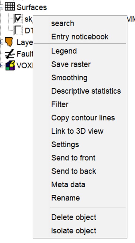
Use the right-click context menu to open the Settings for a loaded elevation grid. You will find various setting options that facilitate a terrain analysis. Explanations can be found in the thematic context under Visual evaluation. You can edit the grid with the section Editing. For the explanation of the general functions on SubsurfaceViewer objects, follow this article.
**The function Copy contour lines can be used to transfer height information and structures from raster data into a Geometry2D object. This means that you copy contour lines, which you can use for editing Structure Maps. Depending on the raster resolution, the isolines are stepped. We recommend performing a Smoothing before creating the Contour lines.
Note: We generated the elevation model shown from the ATKIS®-DGM1 data (source) of the Vogelsbergkreis. {.is-info}
¶ Visual Evaluation
¶ Contour lines
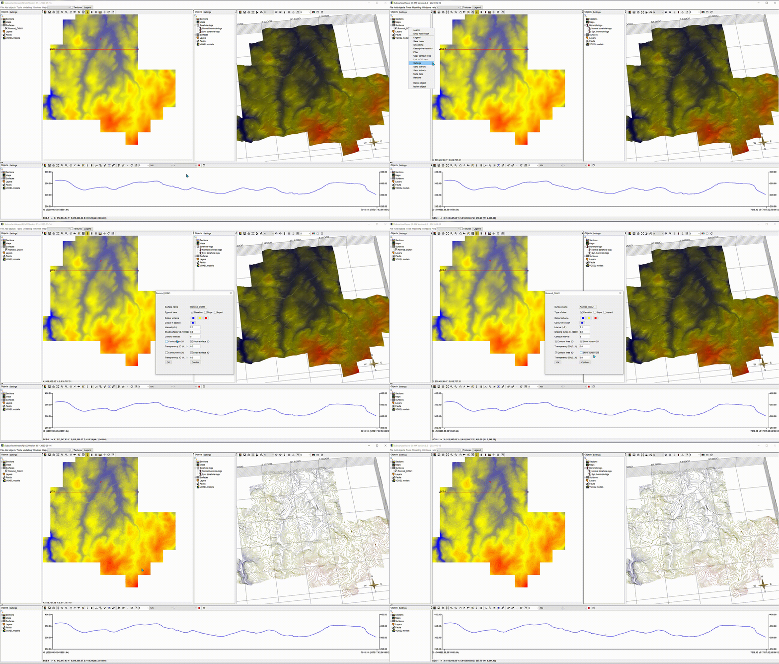
The display of contour lines can be activated in the Settings with a value in metres. As soon as the calculation is completed, you can individually adjust the representations of the lines and the surface and in context for 2D and 3D with the corresponding checkmarks.
¶ Shading
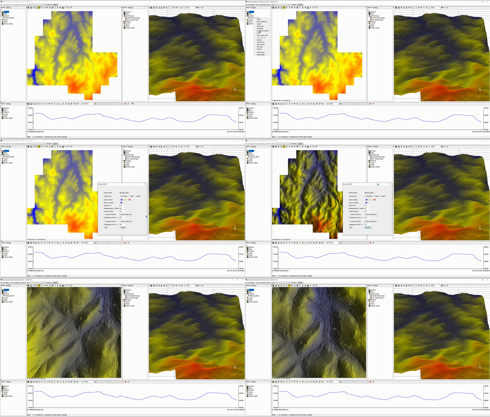
Elevation grids can be shaded with a factor that terrain features can be recognised. This can be advantageous if you want to map surface layers and certain terrain structures are typical for this purpose. The shown DTM (Digital TerrainMmodel) has been created from the ATKIS®-DGM1 data. How to do this in SubsurfaceViewer and where you can find the source for the data is described in this article.
¶ Slope and Aspect
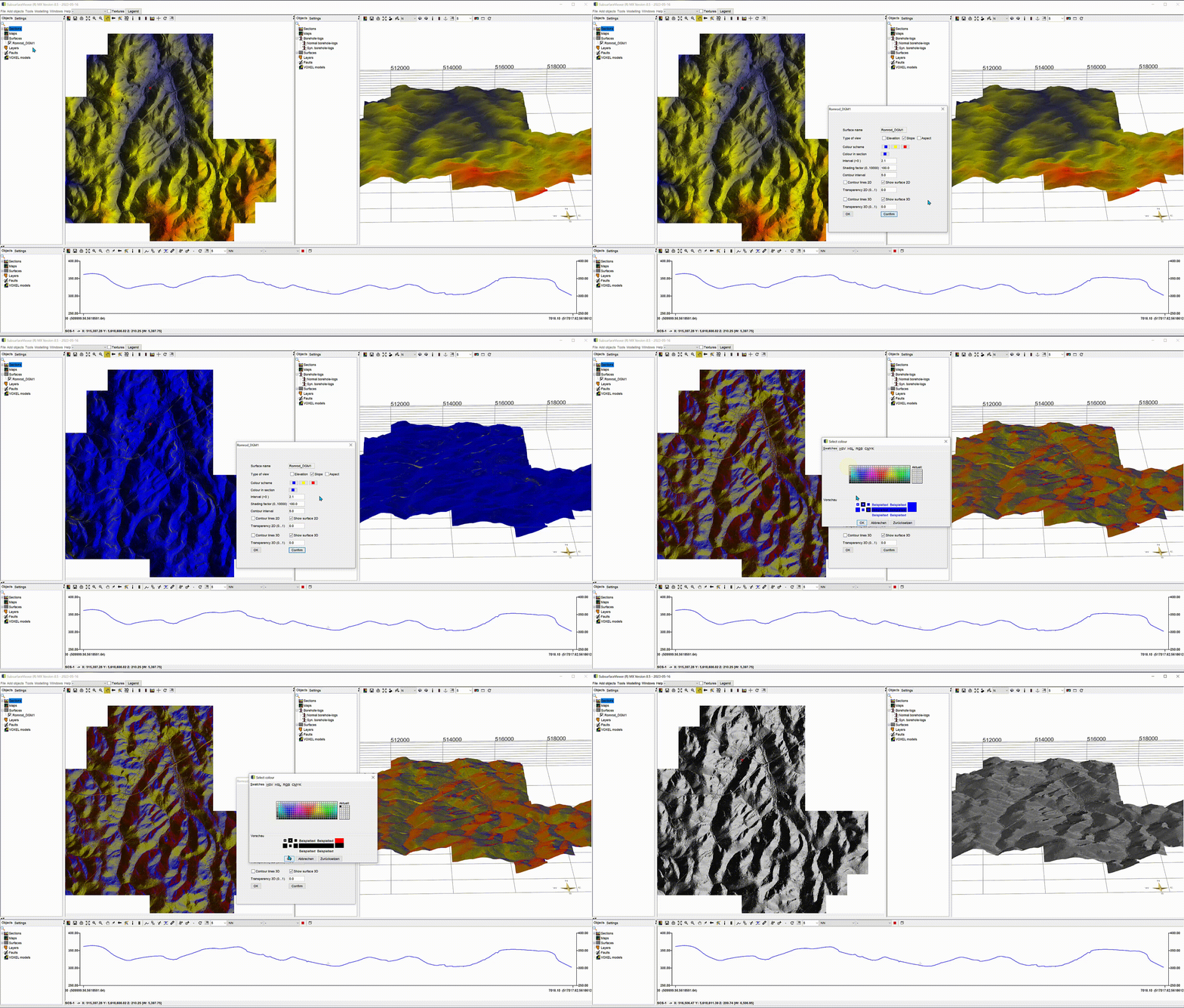
You can change the representation of rasterised terrain models according to slope and slope direction. These applications can be helpful, in connection with information on landslides or flow directions of surface water during heavy rain. From this, indications regarding recent geological units (cover layers), erosion processes or risk analyses could be derived.
¶ Height Grid with a Topographic Map
If you need a topographic map in the project, load it and project it onto the elevation grid. For more information on loading raster maps as images, see this section.
The map shown below is a section of the DTK100 (WMS service) from the Hessian State Office for Land Management and Geoinformation and is available here for download via GIS. For the representations in SubsurfaceViewer, the map has been externally cropped to an area and uploaded here as an image with accompanying world file.
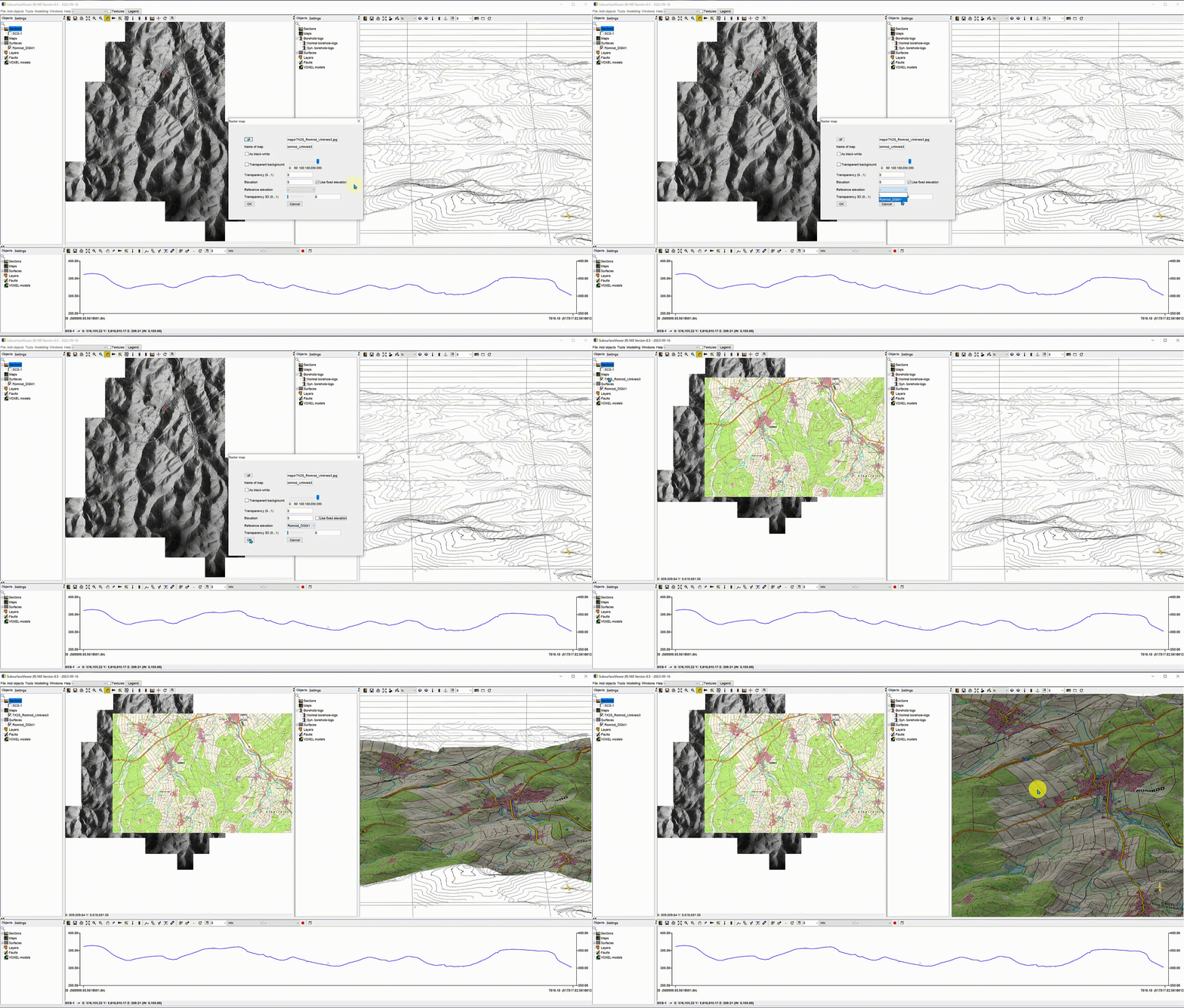
If you have a georeferenced satellite image (source: Google), you can load it in the same way. You can switch certain colour values transparent via the Settings of the topographic map, so that a favourable display of all information is possible.
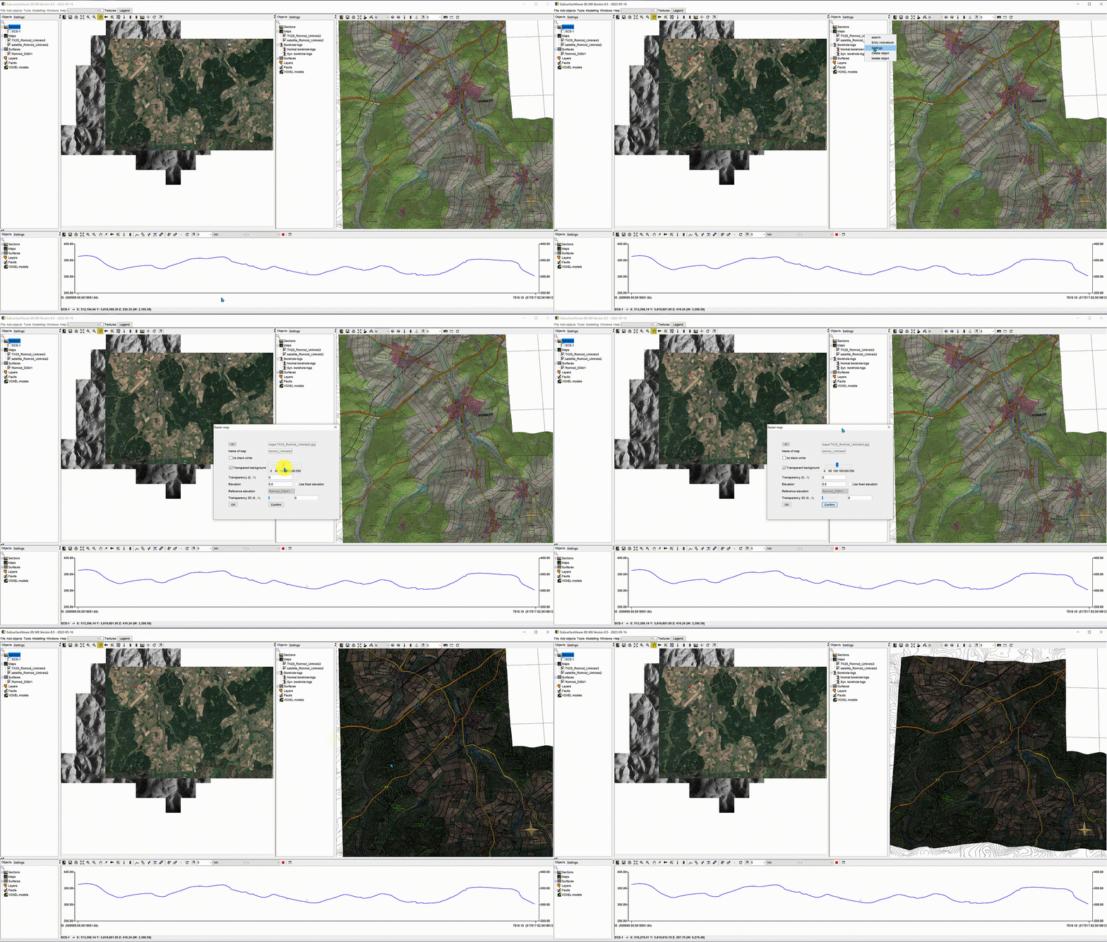
¶ Editing
¶ Smoothing
Use this if you want to use the height information and structures of a raster for a Modelling with Structure Maps. Extract isolines from the raster and use them further. If the grid is not smoothed, the isolines may look stepped. This happens if you want to extract Boundary Raster from a Filtered Voxel and use it as the basis of structural map modelling.
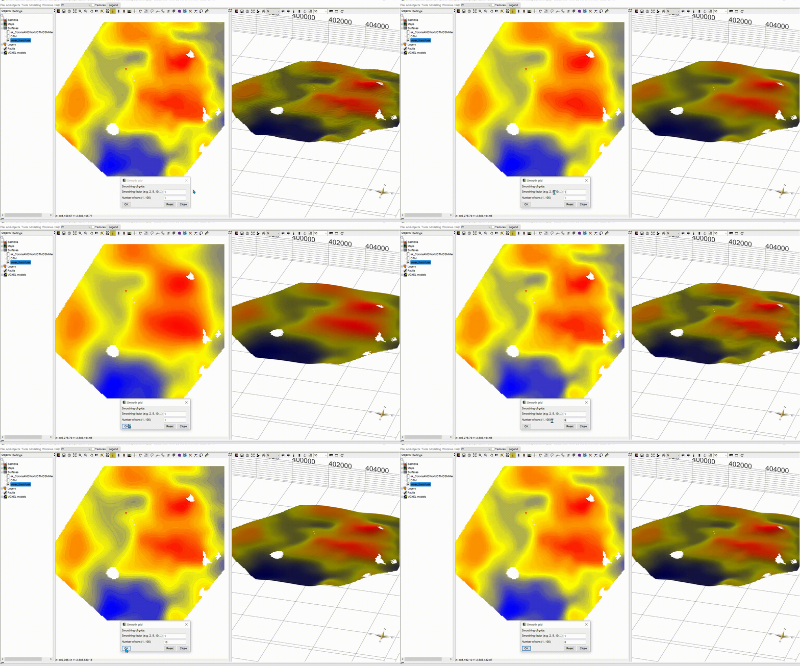
If you select Smoothing from the context menu, a window opens with two input fields:
- smoothing factor
- number of runs
*Smoothing is a moving average calculation.
The Smoothing factor determines the field size around a cell in whose content the moving average is to be set. The field size is the number of cells in each direction around the target cell. If you select a field size of 10, 10 cells to the right, left, top and bottom will be used for a mean value calculation.
A number greater than 1 for Number of runs will cause all smoothing to run multiple times on the raster data created. A previously smoothed raster is smoothed again and the result goes to the next iteration step and so on.
Confirm the settings with OK. The window remains open as long as you do not close it. With Reset you can go back to the original grid. With Save raster in the object context menu you can export the edited raster.
Note: To preserve the structure of a surface, it is best to choose a smaller smoothing factor (e.g. 1, 2) and use a higher number of iterations (number of runs). {.is-info}
¶ Filter and Analyse Elevation Rasters
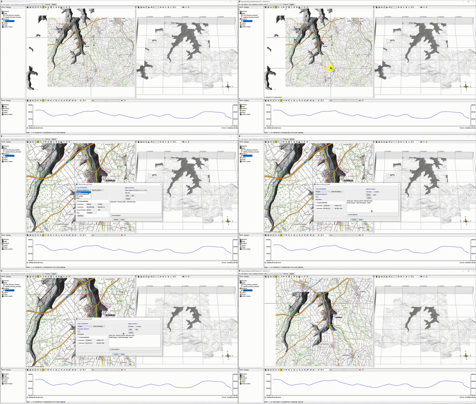
For height grids, you also have the option of viewing the descriptive statistics of the grid and filtering by values or other geometries via the right-click context menu. If you retrieve the descriptive statistics via the filter, you will get the one that relates to the filtered data.
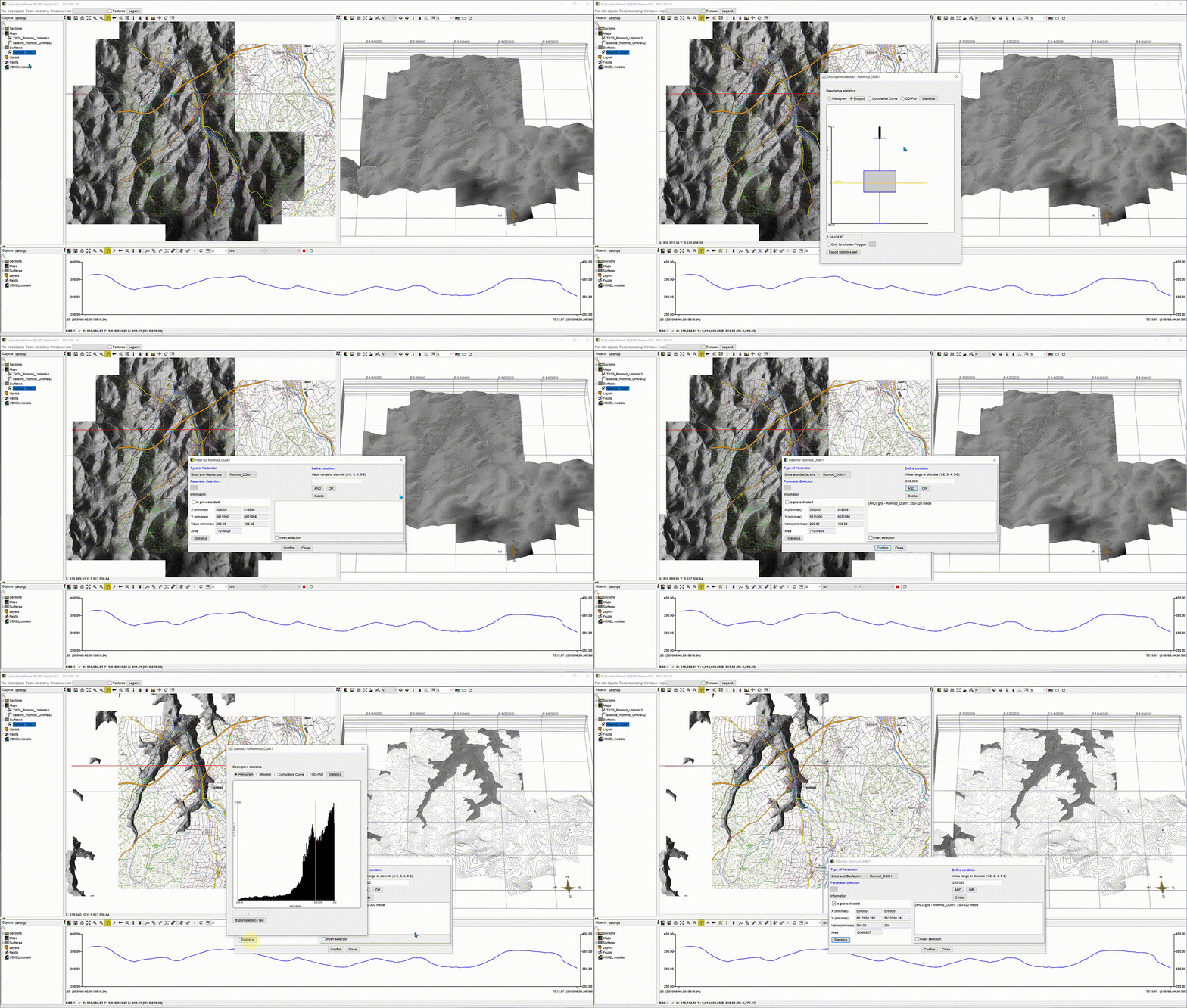
The filter can become arbitrarily complex with AND and OR links, which can be conducive to spatial analysis due to the great flexibility. For more information on the filter, see this article.
¶ Convert Filtered Raster Data into a TIN
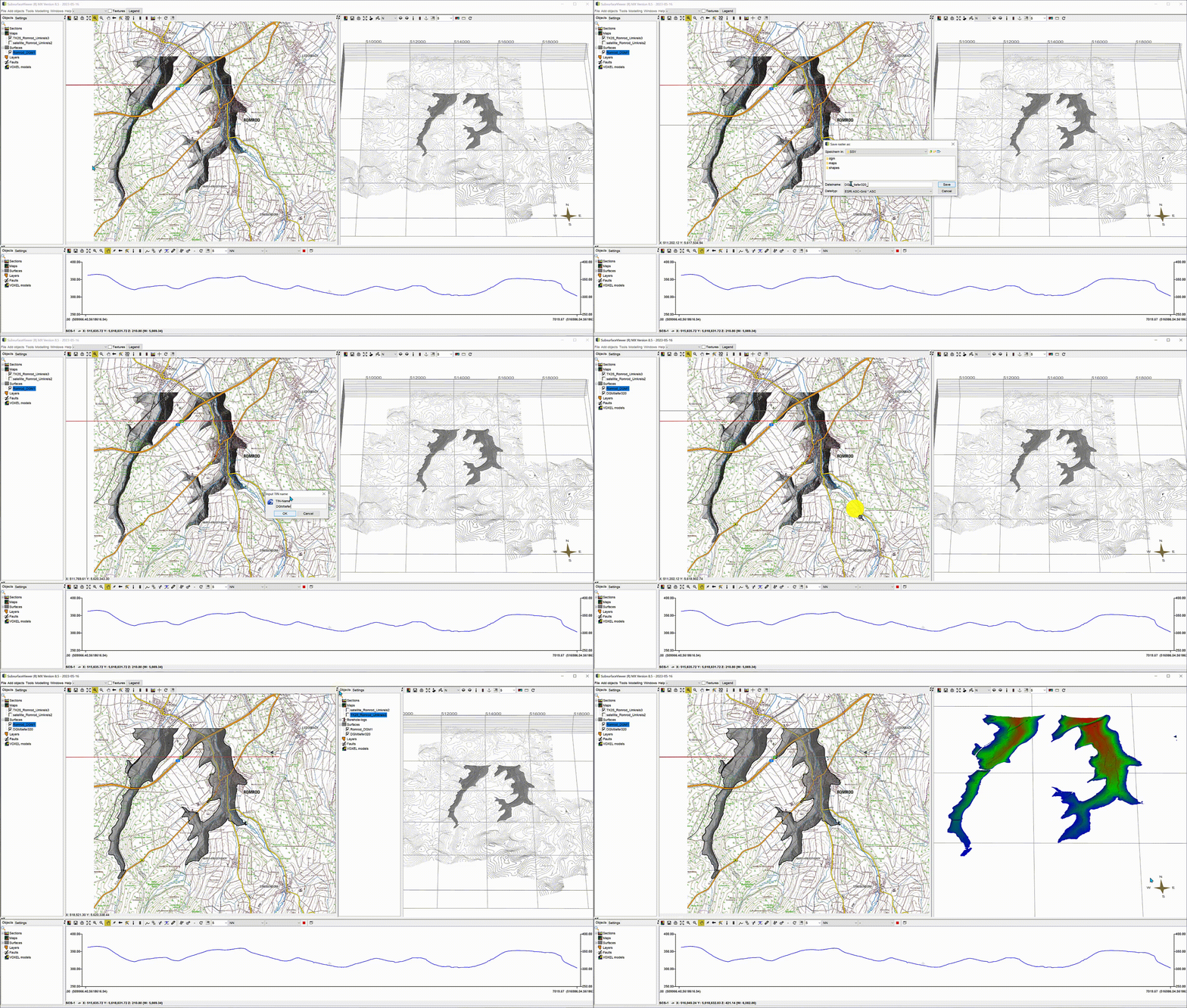
If you want to convert certain raster data into a triangulation, do this with the following workflow. The same way is possible with the full raster, in which case you do not need the first step.
- After you have made the correct filter setting, save the selected raster to its own file via the right click context menu Save raster.
- Create a TIN object as described here and load the grid as a source for triangulation.
- If you need the result in an external programme, you can export this TIN into the formats described here.
Note: With a trick you can extract polygons of certain filtered elevation grids. You will learn this when you start modelling with SubsurfaceViewer.
{.is-info}