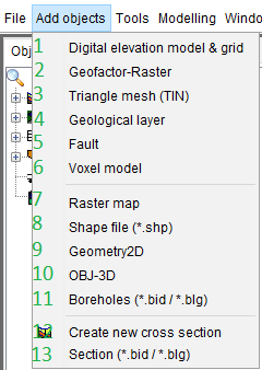
The menu item add objects summarises options for adding different (geo)data to the project.
¶ 1. Digital elevation model & grid
Here are more information about the object-functions: height raster.
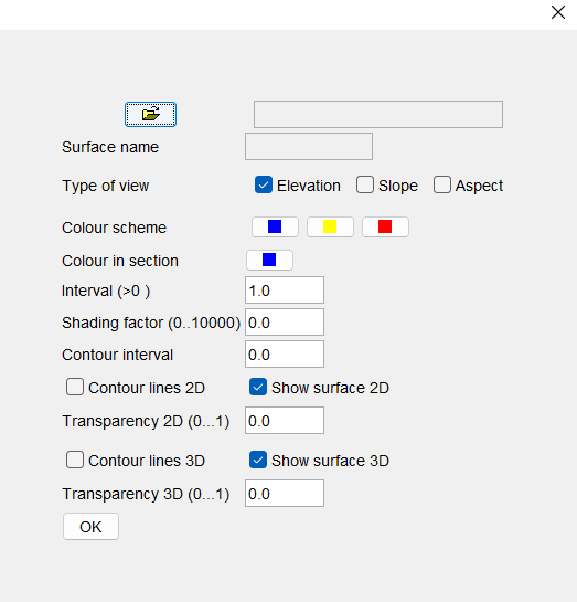
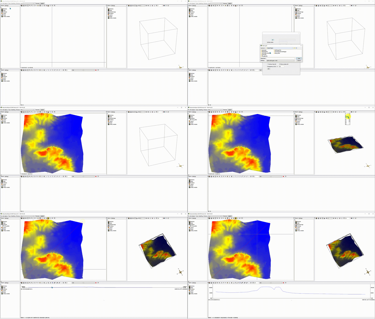
Under Digital elevation model & grid a new model or grid can be added. Please note the possible formats for raster files. Go to the location where the corresponding model is located and determine the type of view, the colour scheme, the colours of the sections, as well as the transparency and the contours of the lines in 2D and 3D. You can do this later by calling up the object settings in the right-click context menu. The advantage is that here you still have some analysis options to analyse the terrain in more detail. With the elevation raster you can carry out further analyses by using a filter and/or by simple descriptive statistics on the raster contents.
¶ 2. Geofactor-Raster
Here are more information about the object-functions: geofactors.
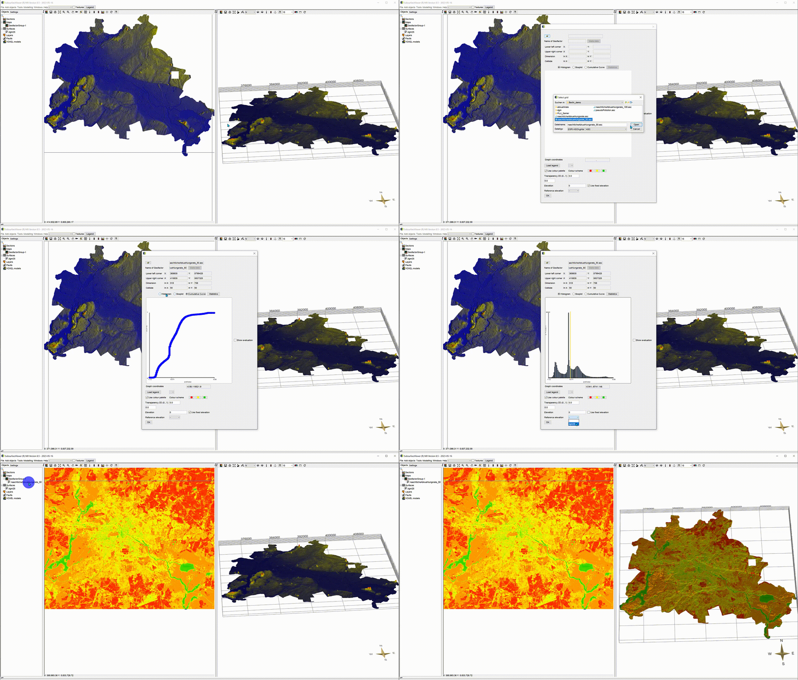
Geofactors are usually data that assume certain values at XY locations. This can be, for example, a hazard potential for landslides, an average concentration of a raw material or a pollutant, a groundwater protection map with a classification, a soil liquefaction potential for earthquake magnitudes or similar. Geofactors in SubsurfaceViewer must be loaded as rasters. So the same formats are valid here as for rasterised surfaces (Formats). Adding a geofactor raster works in the same way as for the elevation raster. However, you have some other settings available here, as geofactors are also part of the implemented SMCA module (Spatial Multicriteria Analysis) (Multicriteria_decision). Independent of the SMCA module, geofactors can also be classified (evaluated) individually and immediately during loading or via the Settings call.
You will see the information on the geometry, the coordinates of the lower left and upper right corners, the cell size and the dimension at the top when loading and in the Settings. These details are decisive for an automatic assignment of a geofactor into a subfolder. When loading, those geofactors are automatically assigned to the same subfolders that also have the same dimension and cover the same region. This will be useful for the correct use of the SMCA tool.
Furthermore, three graphical representations of the descriptive statistics - the histogram, the boxplot and the cumulative curve, can also be displayed. At the bottom you have the possibility to change the colours of the grid and the transparency. In order to be able to display geofactors in 3D, you must specify a height reference, i.e. a loaded surface or a fixed value, similar to topographic maps or shapes. You can also load legends via the settings if you do not like the standard option of colouring via the colour palette. The legends should be in the format *.BELEG, *.VOLEG or *.PALEG. More information on this can be found in this article: formats.
In the example below, a DTM from the ATKIS®-DGM1 of the geodata server FIS-broker der Stadt Berlin vergröbert verwendet (Auflösung 25x25 Meter) and a raster of the nocturnal cooling rate, coarsened also 50x50 metres cells also from FIS-broker, was invited as geofactor raster.
If you want to know how the ATKIS® data in XYZ format can be processed into a DTM in SubsurfaceViewer, you can read this article: advanced functions - raster.
¶ 3. Triangle mesh (TIN)
Here are more information about the object-functions: triangulated areas.
Using this function, a new, empty TIN-Object is added. The TIN is located under "Surfaces" and is given a name. The options for editing a TIN are revealed by right-clicking → Extra Functions. There are four options for filling the still-empty TIN with data.
Attention
Before a TIN object is created, the input of the minimum point spacing, which is set in the project settings, must be considered. Points with distances below this minimum are ignored during the interpolation. This ensures that the triangles do not become disproportionately small at some points in the model.
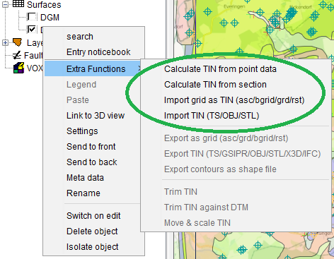
- With Calculate TIN from point data, a TIN surface can be calculated from various file formats with XYZ point data.
- With Calculate TIN from section, surfaces can be modelled from layer bottom edges/lines that are used within profile sections for interpolation. The vertices of the constructed lines are used as input for triangulation. The lines must have the same name in each constructed profile section, which is then selected in the Line name in sections field. Subsequently, each line vertex in these sections is used to calculate a TIN object from them.
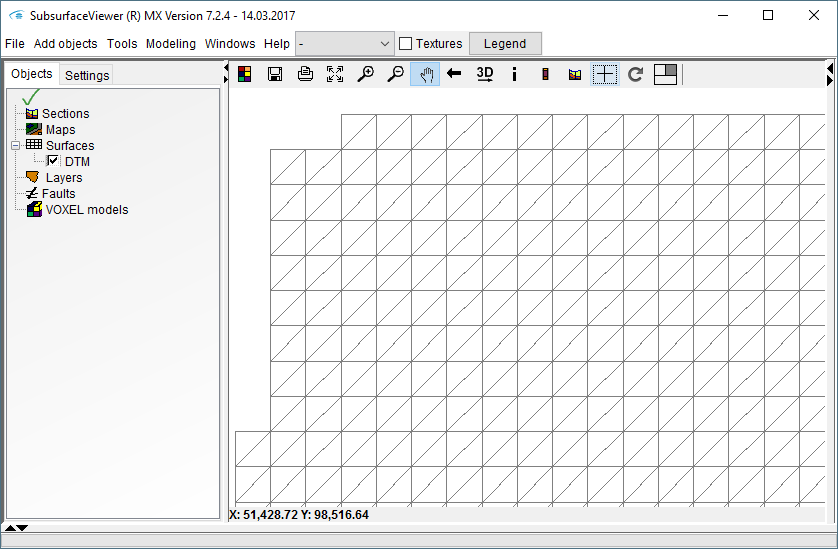
- With Import grid as TIN the information from grid files is loaded into the TIN object. For the conversion of this uniform grid data, two triangles are formed for each cell of a grid. For this, the built-in algorithm has two options - left lower and right upper triangle or left upper and right lower triangle. Therefore, the transformation is not unique. The following figure shows the scheme of the second option.
- With import TIN, TIN surfaces or shells can be loaded that were created in another software, for example in GOCAD.
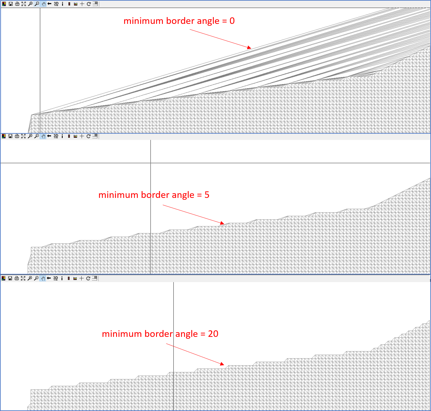
In addition to the options for smoothing and refining, a minimum border angle can be entered. If elevation data is available with an irregular envelope, it may be helpful to assign this minimum border angle. By default it is set to zero and can be changed from 0 to 44.99 degrees. The effect of the selected boundary angle is very strong in some cases, especially if the point envelope is irregular or meandering. In the following figure, a regular DTM XYZ file was used for triangulation, where the edge is not square. The edge angle dominates the surface edges considerably.
¶ 4. Geological layer
Here are more information about the object-functions: geological layers.
Geological layers in SubsurfaceViewer always consist of a layer top and bottom. Open sides are automatically calculated to close the layers at area boundaries in the block.
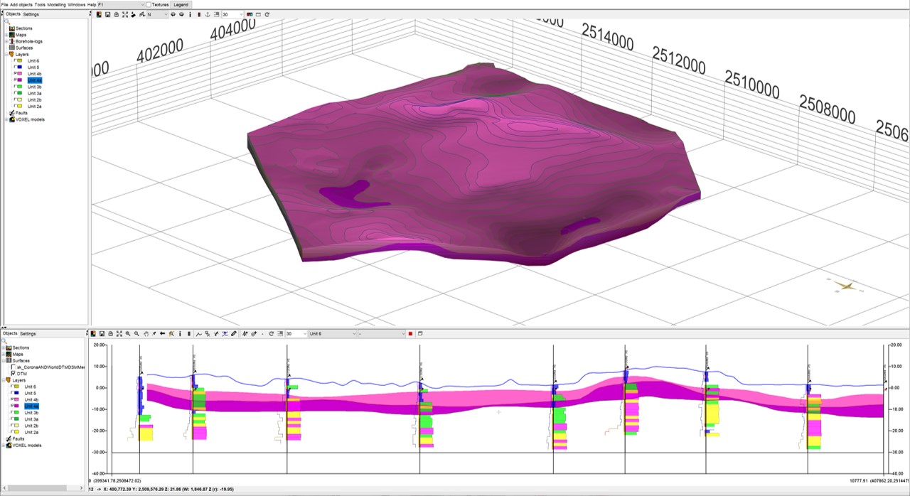 To create a geological layer object, the [GVS file](/en/ErsteSchritte/Projekteinstellungen#gvs-file) and the [legend file](/en/ErsteSchritte/Projekteinstellungen#legend-file) must be stored in the project settings. You also do this with the [project settings](/en/ErsteSchritte/Projekteinstellungen). Then *add objects* → *geological layer* opens a drop-down menu in which the geological layer from the GVS file is selected. If no GVS file is loaded, an error message appears.
After a layer has been selected, an empty object appears in the object tree of the 2D map in the layers folder. Its icon contains the colour defined in the GLEG file. If no colour is associated, the layer object is grey.
If the structural model was created in another modelling programme, it is possible to import the top and bottom of the layer from grids or GOCAD TINs by right-clicking → Extra Functions. This enables the visualisation functionalities of the SubsurfaceViewer for third-party models. The procedure for an initial construction of a layer spread within a geological layer object, as it is necessary when modelling a structural model in the SubsurfaceViewer, is described in Define layer spread.
¶ 5. Fault
Here are more information about the object-functions: fault.
A fault is a tectonic divide along which geological layers shift against each other.
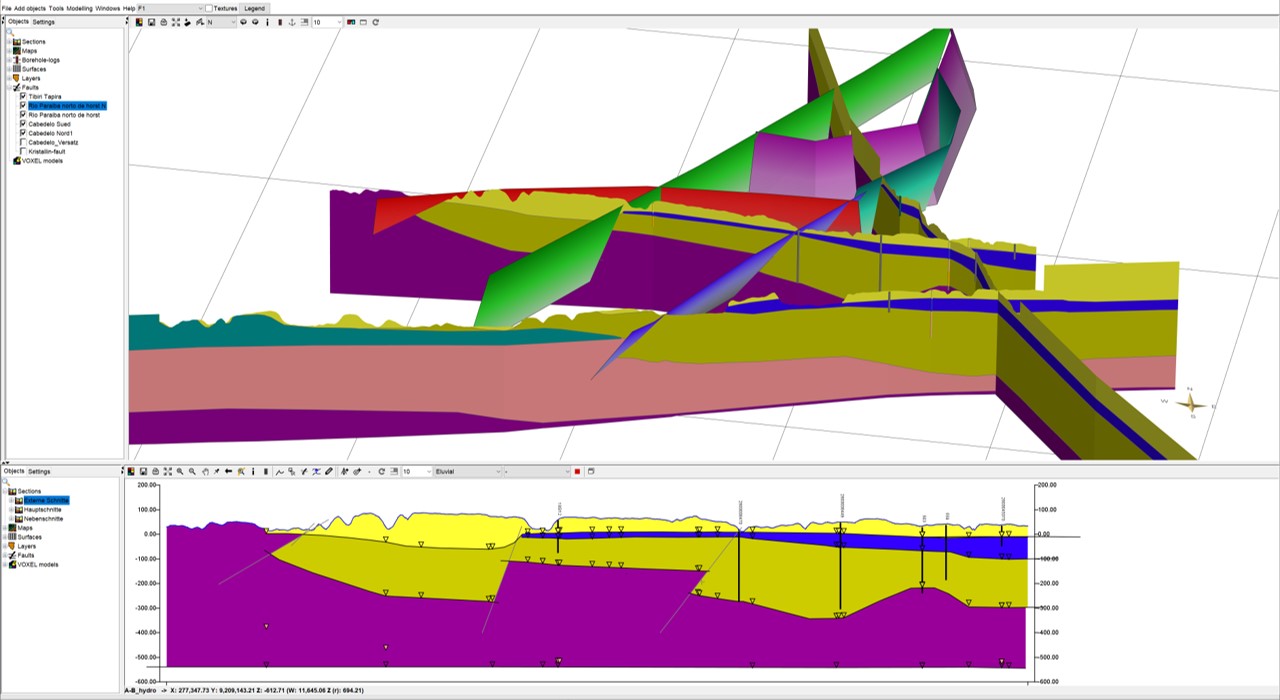
The SubsurfaceViewer can implement faults in the form of triangulations. As with triangulated surfaces, an empty object is created for a geological fault, which can then be filled with right-click → Extra Functions. You can calculate the fault directly, load a Gocad TIN object as a basis and also export a fault in various file formats.
If you do not want to load the disturbance from outside, but construct it yourself, you can read the above-mentioned article on object functions.
The SubsurfaceViewer is, so far, specialised for 3D mapping of lock sediments. Fault systems have therefore not been fully developed. Although you can construct and load them. Also the profile sections show layer polygons adapted to the faults when constructing the lines. However, they are not included in the regular layer calculation. When exporting the profile sections to 3D shapes, they are ignored. It is recommended to use another specialised programme if you want to use the SubsurfaceViewer. You are welcome to write to us if you feel that the extension should be considered in our further development.
¶ 6. Voxel model
Here are more information about the object-functions and implementation of voxel models: voxelmodel.
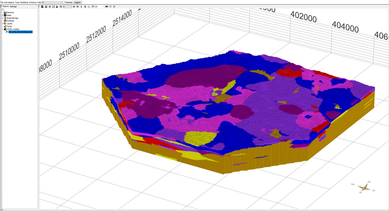
Voxel models are space-filling models that depict a cuboid around a certain XYZ coordinate, which is assigned a value. They are therefore volumetric models. In SubsurfaceViewer they are mainly used for the interpolation of parameters or to be able to volumetrically map layer models.
¶ 7. Raster map
Here are more information about the object-functions: maps.
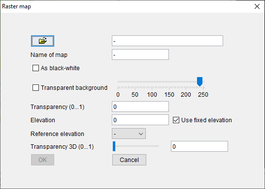
With Raster map, a rasterised image file, for example a topographic map in TIF format, can be loaded into the project. The map can be converted to black and white and/or the background can be set to transparent. The transparency of the entire map can be set separately for the 2D and 3D views. A height can be selected for the map that is relevant for the view in the 3D view. A fixed elevation value (Use fixed elevation) in metres above sea level can be entered, or a reference area can be selected (Reference elevation).
¶ 8. Shape file (*.shp)
Here are more information about the object-functions: shapes.
ESRI shape files can be loaded as point, line or polygon shapes as 2D map objects. 2D and 3D shapes for lines and polygons can be loaded. In both cases the objects are initially displayed as 2D lines or polygons in the map view. A 3D view therefore requires the use of the right-click context menu and the 3D view function located there.
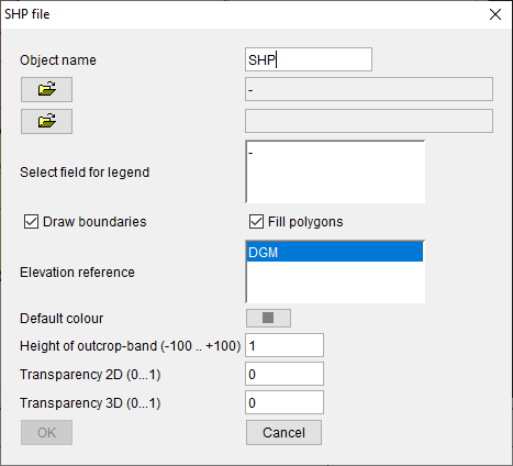
The elevation of 2D polygons can be referenced by a grid or a TIN (Elevation reference). The polygons are displayed in the 3D window with the respective surface, for example with a digital terrain model (DTM). If you use 3D polygons, they are given the elevation from the file and the transmission of an elevation reference is inactive. If you want to see polygon shapes as textures on your elevation model, you should load them as 2D shapes.
In the profile sections in the 2D cross-section view, the polygons are displayed as a band on the assigned surface, for example "lying" on the DTM. The band has the thickness in metres entered under height of outcrop-band. You can find an example in the article on object functions linked above.
The definition of shape-files is in ESRI. More details about it can be found here: http://www.esri.com/library/whitepapers/pdfs/shapefile.pdf
¶ 9. Geometry2D
Here are more information about the object-functions: Geometry2D.
Geometry2D is a SubsurfaceViewer specific object for drawing lines and polygons. This object is mainly relevant for the construction of layers via Structure Maps.
It can also be used for quick filter 2D and 3D raster data or for marking as an aid during modelling.
First, an empty object is created via add objects, which can be filled or edited with data via the right-click menu. You can load polygons and lines from shapes and edit them in this object. The Geometry2D object can be exported as a shape (ESRI).
¶ 10. OBJ-3D
Under this, data from other 3D design programmes can be loaded in *.OBJ and *.STL formats.
For example, you can add 3D city models to a created geological model and view them in the 3D view. You must either ensure that the loaded object is georeferenced or that you have created your model with relative coordinates that match the OBJ-3D object you are loading.
Please note that OBJ-3D objects in SubsurfaceViewer only have a 3D view. They are not visible in profile sections and in the 2D map, which is why they only appear in the 3D object tree.
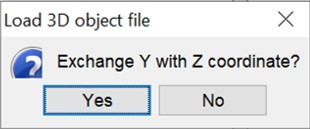
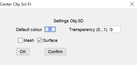
When loading, you will be asked if you want to convert the Y-axis to the Z-axis. This must be confirmed with Yes for a correctly oriented view. You have the possibility via the right click menu -> settings of the object to switch between surface and mesh for a view as well as to select a general colouring of the surfaces to which no further colouring is assigned in the file. You can set the transparency of the surfaces with values between 0 and 1.
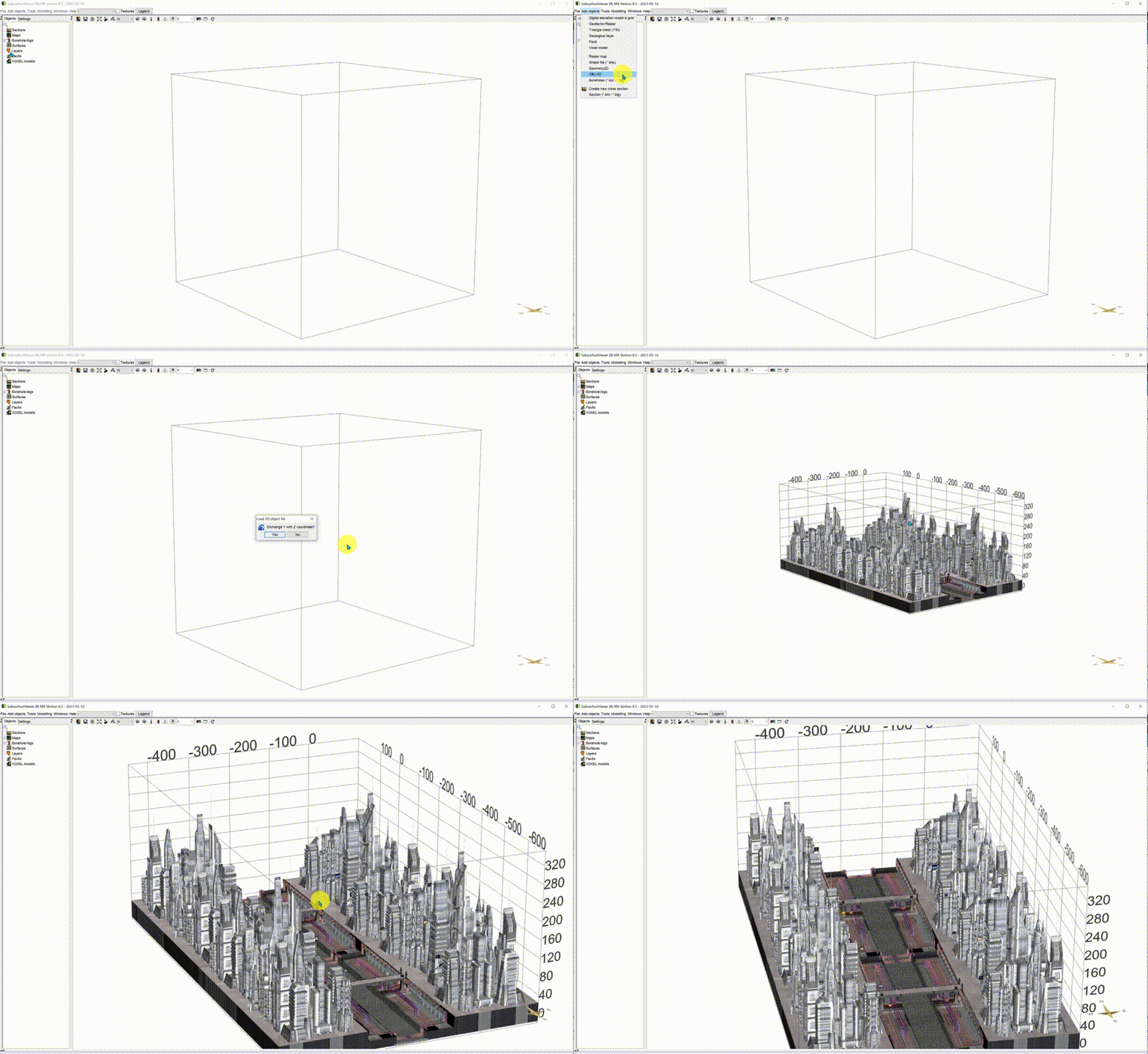
In the following example, we used a fantasy-example. You can download it for free here.
¶ 11. Boreholes (*.bid/*.blg)
Here are more information about the object-functions: boreholes.
Boreholes in SubsurfaceViewer are always vertical logs, as this has been completely sufficient for our circle of users up to now. Logs with deflection and skew or horizontal course cannot be displayed via this function. But if you absolutely have to, and how you could achieve this with tricks and manual work as well as a few compromises, we have linked here. Feel free to contact us if you think functionality should be expanded here for our further developments.
Borehole data are loaded into SubsurfaceViewer via at least two files. A master data file as *.bid and a description file as *.blg. You load the master file with borehole master data and the layer descriptions with layer description. Both are simple tab delimited ASCII text file formats. Loading boreholes into the SubsurfaceViewer system results in borehole objects (under maps) and the associated borehole logs.
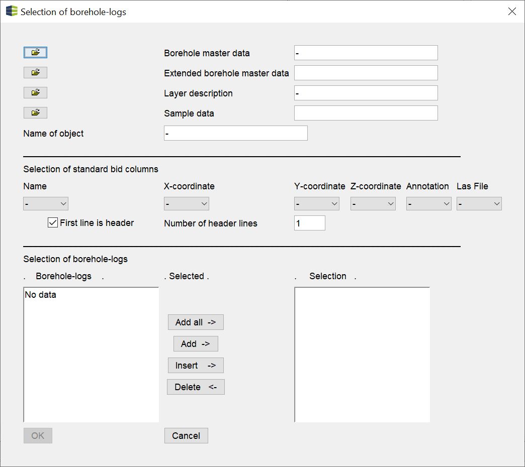
In addition, under Extended borehole master data you can load a *.ebid file that separately contains metadata about the boreholes, such as date, drilling company, quality check. Under Sample data you can also load a *.plg, which still contains numerical measured values for certain depth intervals at the respective drilling points.
In the section below, you can select the columns from the *.bid file that contain the relevant information and specify the number of headers.
All entries will be visible in the list on the left when loading a *.bid. With a marker, you can load the selected holes with the add -> button. You can select all the boreholes with add all ->. Selected boreholes appear in the list on the right. With insert -> a borehole is inserted at the position in the list where you are currently with the mouse. This is only for your overview. With delete -> you can remove selected holes from the list.
Note: You can load the master data of field data (*.bid) without any additional information. Then you can display the locations with their names in the 2D-View as well as in the profile sections. You will not receive any depth information.
If you have already loaded layer information for this *.bid through the file in the project settings, you do not need to load this *.blg file a second time at this point. The file with the layer information in the project settings is interpreted as globally valid and is always queried for keys.
Note:
The SubsurfaceViewer needs a dot (.) as decimal separator for coordinate or height values, as here in the columns B to D, otherwise an error occurs when loading the drilling data.
Table programmes set to German (such as MS Excel), on the other hand, use a comma as the decimal separator by default. Therefore, either the corresponding export setting must be selected or the setting of the programme must be changed to comma as decimal separator.
¶ 12. Create new cross section
Here are more information about the object-functions: profile sections.
This tool is used to create a new profile section. A name is given and the empty profile section can be found under "Sections". An example can be found here.
¶ 13. Section (*.bid/*.blg)
Here are more information about the object-functions: profile sections.
In contrast to create new cross section, Section (*.bid/*.blg) can be used to create a profile section in which boreholes are already included. The window for creating the object corresponds to the one when adding a borehole point map (Boreholes (*.bid/*.blg)). The course of the profile section is created along the order of the boreholes in the right-hand list Selection.