You load geological layers in the Mainmenu under Add objects -> Geological layer.
Note: You must have loaded a GVS file in the project settings before you can use this function.
Note: You do not have to have created a geological layer if you want to construct it manually in profile sections. For the construction in the profile sections you need the loaded GVS file. {.is-info}
A geological layer always consists of three elements:
One triangulation each of the bottom edge and the top edge of the layer, if calculated.
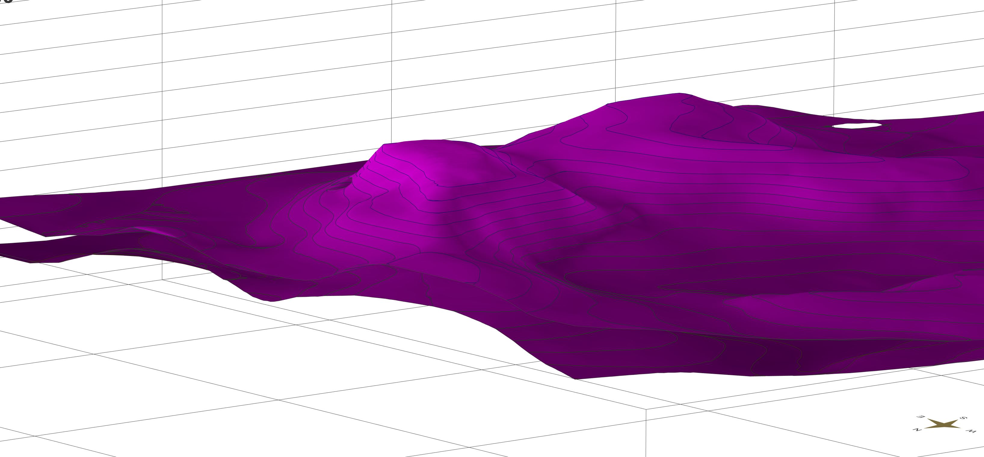
Note: The pages you see to display a 3D layer block image are automatically calculated for the display. They are not part of the object as it is saved and loaded.
Important:
In SubsurfaceViewer you construct geological layers via the layer bottom edges. The outer edge of the layer results from the boundary polygon. The nodes of the boundary polygon receive the heights of the overlying layer lower edge or of the DTM, if the outcrop of the layer lies at the terrain upper edge. The top of the layer is calculated from the sum of all the lower edges of the layers lying directly above this layer.If, you add layers from external sources, you can load the layer top separately instead of calculating it.
¶ Create geological layer
Select a layer object from the dropdown list that opens for you and contains names of the defined layers from the GVS file and confirm. You can load a layer once at a time. The object is added to the object tree of the 2D-View under the category Layers.
This object is initially empty, if it does not have any layer polygons or triangulated surfaces.
To complete a geological layer, there are various ways, which we outline below and to which you are directed in each case to one of our How To pages, where we have compiled modelling procedures in their entirety.
Note: The triangle mesh is always calculated in SubsurfaceViewer using the Delaunay method. {.is-info}
¶ Create layer polygons
- Construct the layer polygons or borders by hand. Read Define layer distribution.
- Copy the polygons from a geolgical map or an externally created layer boundary into the buffer and from there back into here. Read Shapes.
- Run a triangulation without a boundary and see what boundary results (not recommended).
Note: For step 1. and 2. you have to switch the layer active for editing. To do this, use the right-click context menu in the 2D view object tree and Switch on edit.
¶ Create layer bottom edge and layer top edge
- Construct profile sections and layer polygons. Calculate the layer lower and upper edges with this. Read here: Calculate Model.
- Construct structure maps, layer polygons and optionally profile sections. With these you calculate the layer lower and upper edges. Read here: Modelling with structural maps.
- Import triangulated layer lower edges and optionally layer upper edges into the layers. Layer top edges can be calculated once you have loaded layer bottom edges. Read here: Integrate model data from other sources.
- Import raster-based layer lower edges and optionally layer upper edges into the layers. Layer top edges can be calculated once you have loaded layer bottom edges. Read here: Integrate model data from other sources.
- Import an additional XYZ point dataset for the operations 1. and 2.. Read here: Add scattered data points.
¶ General options
Here we describe the specific contents of the object context menu. For the functions that are generally valid for objects, please read here.
For the functions under Settings and Extra functions we have created separate sub-chapters below.
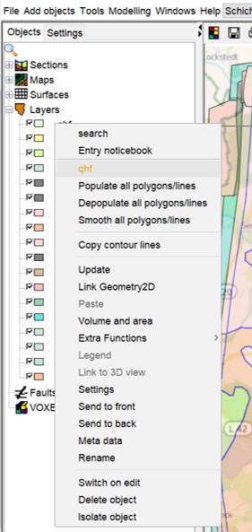
Populate all polygons/lines: Allows you to increase the node density for all layer boundaries to a target distance in metres.
Depopulate all polygons/lines: Allows you to thin out the node density for all layer boundaries to a target distance in metres.
Smooth all polygons/lines: Allows you to increase the node density for all layer boundaries to a target distance in metres, uses a spline algorithm to make the line more curved.
Copy contour lines: This copies created isolines of the layer bottom or top edge into the buffer for reuse. You must have calculated contour lines in Settings beforehand.
Update: This function updates the view of the lines of this layer along the profile intersection in the 2D-View. Read this article to understand what this is for.
Link Geometry2D: This function binds a Geometry2D object to this layer, which provides the information for the surface calculation. Read the article Modelling with Structure Maps.
¶ Settings
The Settings are kept relatively simple. They are visualisation options for the 2D and 3D views of the SubsurfaceViewer user interface.
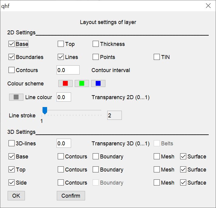
In the upper area are all the options for the 2D view. The 3D settings follow below.
2D:
Determine what you want to see and set check marks accordingly.
- Is it the bottom edge of the layer? --> Base (has an influence on the contour line calculation!).
- Is it the top of the layer? --> Top (has above all influence on the contour line calculation!).
- Is it the layer thickness? --> Thickness (has above all influence on the contour line calculation!).
- Should the layer boundary also be visible as a filled polygon? --> Boundaries.
- Do you want to see the lines of this layer along the constructed profile sections? --> Lines.
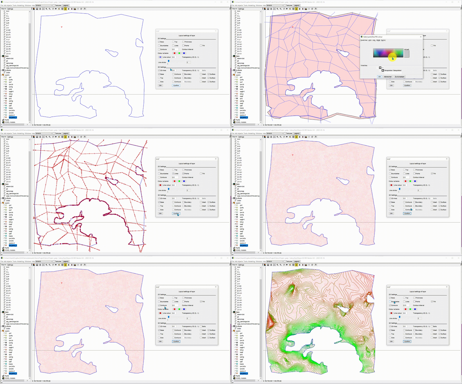
- Do you want to see the height points of the triangle mesh? --> Points (only with active TIN view, see below).
- Do you want to see the triangle mesh? --> TIN.
- Do you want to see the isolines of the layer lower edge, upper edge or the isopaches? --> Contours and Contour interval in metres. The result is conditioned by the setting to Base, Top or Thickness.
The field Colour scheme below visualises the isolines/isopaches with a three-part colour gradient from low to high.
With Line colour you define the colour of the lines in the section gradients (Lines).
With Transparency 2D (0...1) you define the transparency value of the filled layer border (Boundaries), where the value 0 = opaque and 1 = completely transparent.
With Line stroke you can change the line thickness of all 2D-visualised lines in the 2D-view and in the profile section. This allows you to emphasise or visually soften certain layers.
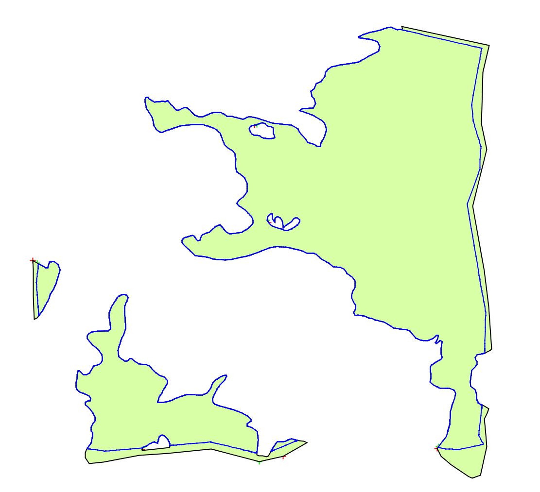
Note: You have certainly noticed that when the layer outline is inactive, a blue outline polygon without fill colour is visible in the 2D settings. This is the outer border of the layer bottom edge after triangulation has been completed. You will see this when a triangulation is present. You can make good use of this outline to detect and check discrepancies or truncations of the TIN compared to the constructed polygon.
3D:
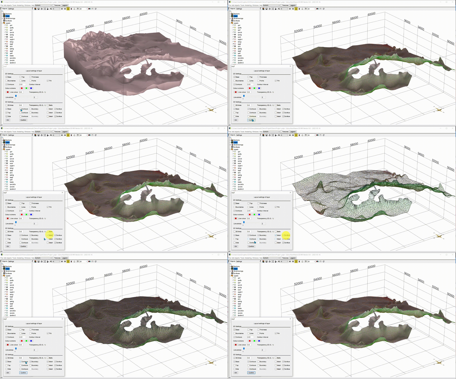
Define what you want to show and hide:
- With 3D-lines you activate the lines along the section courses in 3D.
- With Transparency 3D (0...1) you define the transparency value of the layer surface (Surface), where the value 0 = opaque and 1 = completely transparent.
- If you have calculated isolines, you can activate Belts. Show the surface within every second section between the calculated isolines. Stripes are created. This can be helpful for the interpretation of certain visualisations over several layers or parameters.
Below you can set the visualisation for the top of the layer (Top), the bottom of the layer (Base) and the sides (Side). :
- Contours: Isolines. If you have calculated isolines and have Contours inactive, you will find shading of the layer surfaces based on the isoline calculation.
- Boundary: Shows the layer boundary as a black line in 3D. This is especially helpful when matching layer boundaries with the nodes of the layer bottom edges in the profile sections. Tip: to do this, switch on the cross in the 3D settings.
- Mesh: Shows the triangle mesh in 3D.
- Surface: Shows the filled coloured layered surface in 3D.
¶ Extra functions
Under Extra functions you have calculation functions for the individual layer. Here you can import and export surfaces, add point data to the calculation and evaluate a parameter from the parameter-file *.plg on the layer:
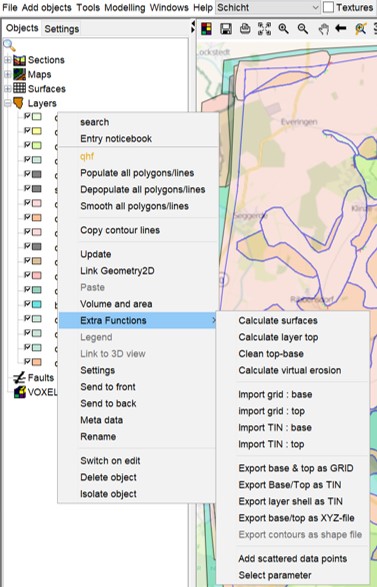
- Layer calculations are available in the upper section. The details of the layer calculations are summarised in this article, so we will only briefly outline the functions here.
Calculate surfaces: Opens the surface calculation of the layer in the full range of functions.
Calculate layer top: Calculates the top edge of the layer from created or loaded bottom edges of the layer. Can be used with imported layer bottom edges.
Clean top-base: Places where the bottom edge of the older layer penetrates the bottom edge of the younger layer are cleaned up by aligning them. A minimum thickness of the older layer is assumed, which you set in Calculation Settings. After the adjustment, the lower edge of the older layer is always at the distance of the minimum thickness below the next younger layer(s) at the affected points. This function can be used with imported layer lower edges.
Calculate virtual erosion: Places where the lower edge of the older layer penetrates the lower edge of the younger layer upwards are cut out.
The import and export functions are self-evident. Read this article on Formats.
With Add scattered data points you can load an external point data set with the absolute heights of the lower edge of the layer for the nodal points that you have set manually in sections or structure maps as well as polygons. These points are included in the triangulation. You will see these points in the Settings with active Points.
With Select parameter you select a parameter from the loaded *.plg-file in the dropdown list that opens.
If values of this parameter are within the calculated layer, a mean value of the data is calculated over the vertical at the parameter XY point. The mean value corresponds to a weighted average over the fulfilling thickness of the individual parameter values.
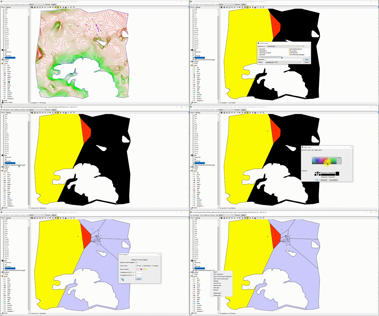
In a pop-up window decide whether you would like to see a Voronoi map for it. You can see the Voronoi map in 2D under Maps. The polygons are trimmed using the defined layer polygons.
You will then be asked for a storage location for the created points. If you define a file name, the weighted layer-internal mean values of the target parameter are written out to you as an XY value table. You can interpolate this point data set in a 2D-IDW or 2D-Kriging run. If this interpolation is to be limited to the layer, export the layer polygon as a shape-file, load the shape-file and copy its contents into the buffer. Then select Trim by polygon in the interpolation algorithms.
¶ General 3D-Settings
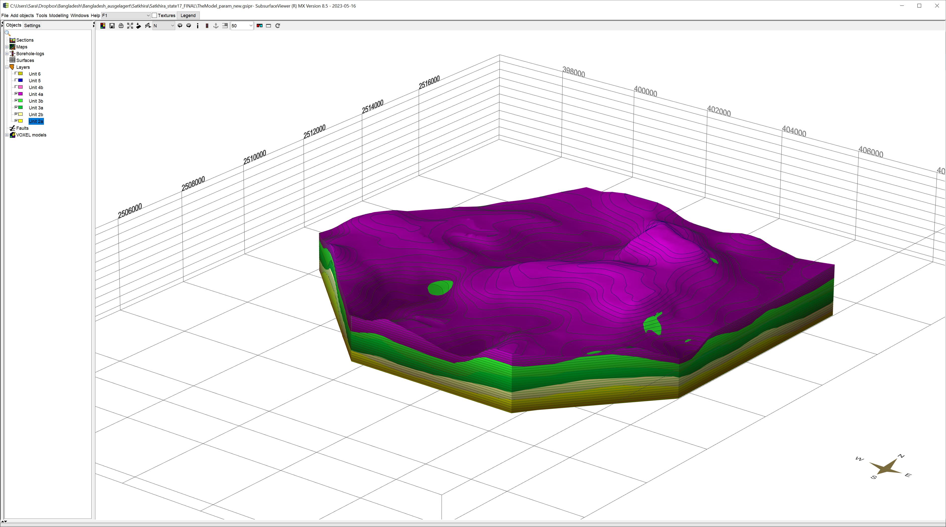
If you click on the symbol  in the object tree of the 3D-View with right click, a separate window opens. This allows you to select what you want to see for all layers at the same time.
In addition, you can crop the model at any vertical layers.
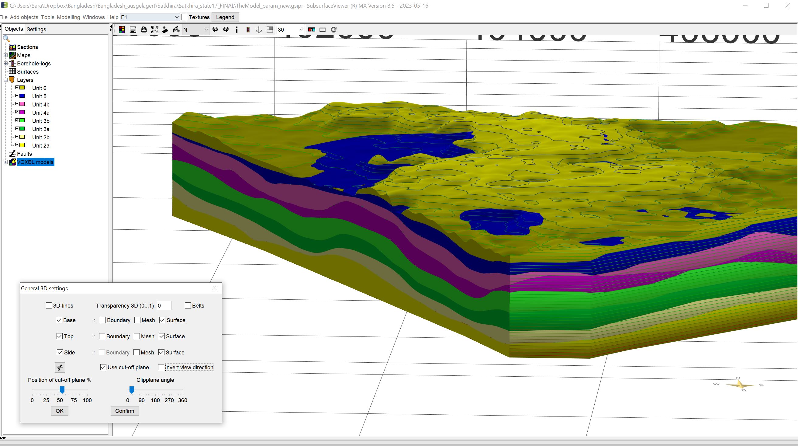
To do this, activate the check mark at Use cut-off plane. With the  tool you set a cut-off plane active. It is initially perpendicular to the viewing beam. With Position of cut-off plane you determine where the dividing line is set that cuts off the model. At 0 % there is no cut and the further the slider is moved towards 100 %, the more is cut off. With Clipplane angle the angle out of the line of sight is set for the cutting plane.
 The
The 