Note:
The SubsurfaceViewer offers 2D and 3D point kriging for interpolation of parameters for geological layer models for unconsolidated sediments. The implementation was project-specific and adapted to the needs of the users, so you will find a deliberately easy-to-understand tool for kriging in specific problems.The application does not, cover the full range of possible kriging methods and options. If you need this, it is recommended to prefer a programme specialised in kriging.
You are welcome to contact us if you feel that we should expand on this topic in our further developments.
You can find the 2D and 3D Kriging option in the main menu bar under the item modelling.
All kriging calculations in SubsurfaceViewer are using the ordinary kriging method. You can work with different variogram models as well as nesting variograms, to make some adjustments to fit the experimental variogram, to check the data for your descriptive statistics, to perform kriging with anisotropy, and to transform data in advance. Cross validation gives you the opportunity to check the goodness of your estimate.
We provide indicator rigging, which can be used as both a threshold or categorical indicator rigging. You can perform median indicator kriging for the limit observation.
Note that we do not deal with kriging theory in the context of this wiki. We only show examples that do not necessarily represent a sensible handling of the input data presented. The examples only serve to explain the functionalities. Nor do we make any recommendations for specific kriging settings or procedures for variogram model fitting. This is dependent on the data set, spatial complexity, spatial distribution and value distribution of the parameters. It is common that the proper use of kriging requires some practice and experience. Fortunately, you can learn quite a lot about this topic through internet research. If you want to go deeper and become more professional in the field of geostatistics, we recommend the site of Prof. Michael Pyrcz, where you can get a lot of knowledge about the whole spectrum of geostatistics. From here you can look for specified applications or Python libraries if you want to work beyond the possibilities of the SubsurfaceViewer.
The kriging functions of SubsurfaceViewer, are well suited if you want to do ordinary kriging or indicator ordinary kriging in the loose solid area to obtain initial estimates of how certain parameters are distributed. If the cross-validation returns good results, use this kriging for further investigations. The interactivity of the variogram generation saves time and is easy to understand. The full evaluation possibility of your result grids with the SubsurfaceViewer is another advantage.
If you open our menu item for kriging, the window shown below appears. On the left side you can load the data and make settings for the experimental (semi-)variogram and the variogram model. Here you start the kriging calculation and the cross-validation. Further down on the left you will find visualisations and options for descriptive statistics. The experimental variogram and the variogram model are located centrally in an interactive drawing field. At the bottom, you will find the advanced settings for variography and kriging with different tabs.
Note:
During the variography and kriging process, many logs and information are written to the info-window. It is recommended to view this to better check the quality of your estimates.
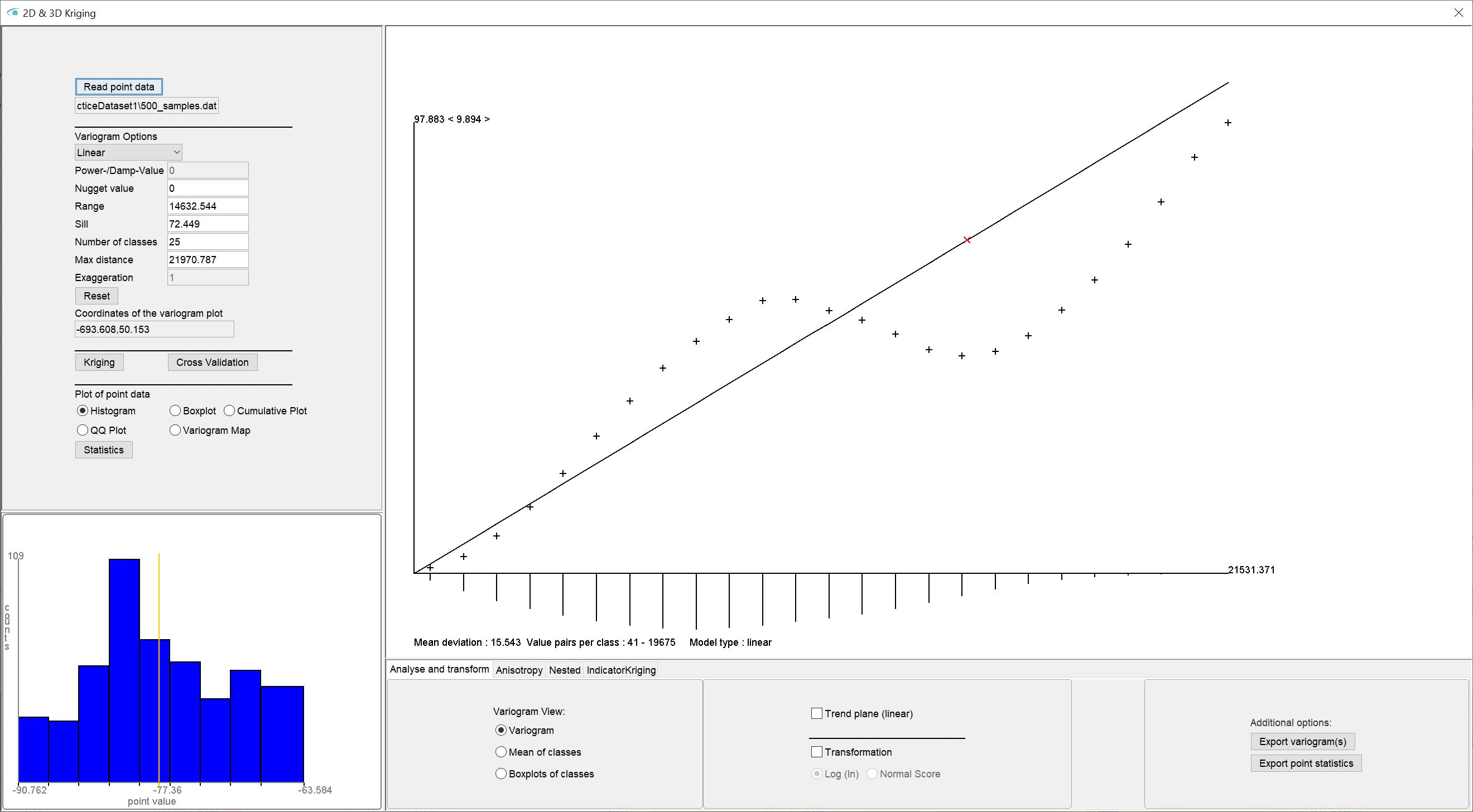
With read point data you load your point data set. The input formats can be found here. As soon as the import is complete, the experimental (semi-)variogram and the descriptive statistics are calculated.
Note: If the data set contains many thousands of points, the calculation of the experimental variogram may take several minutes. It is advisable to reduce the data sensibly and carefully or to use another application.
In the following, this article is subdivided for 2D and 3D together according to topics of variogram creation, options and final kriging calculation:
¶ Experimental Variogram
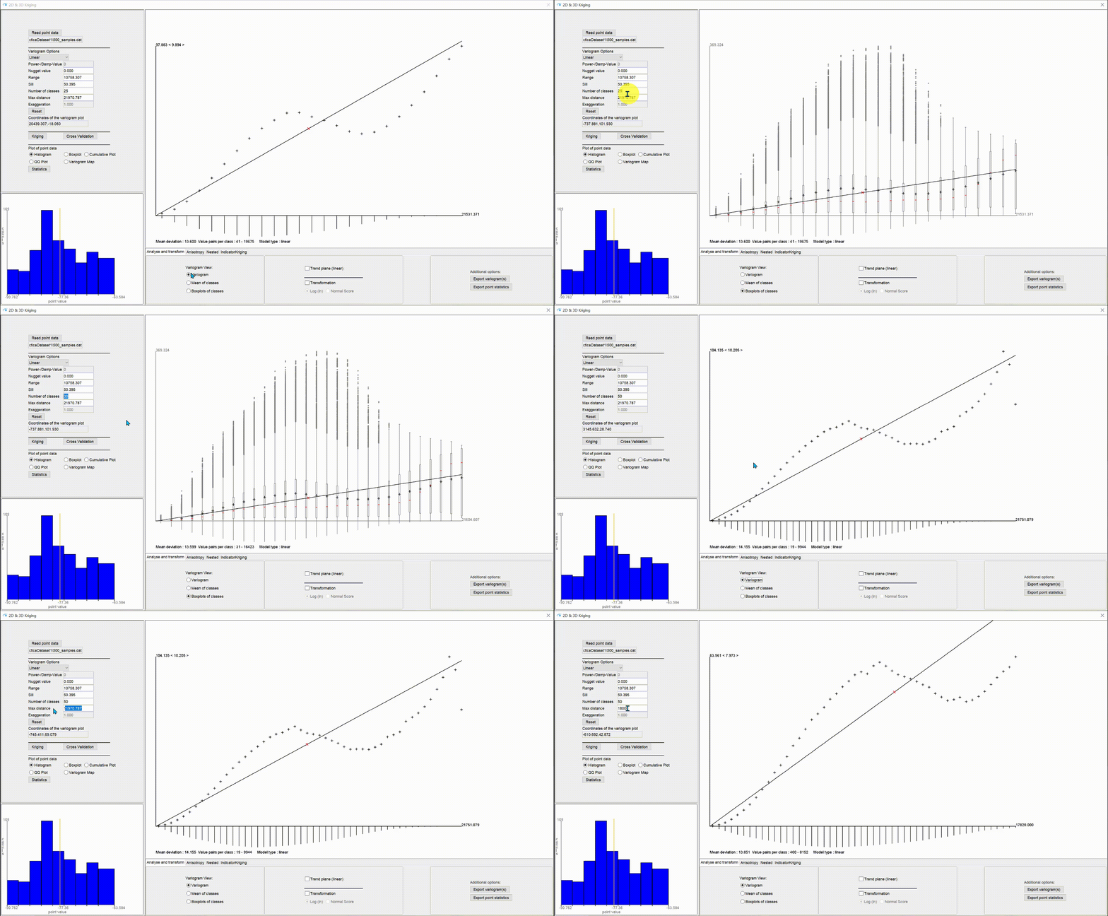
In the central drawing area of our Kriging window you see the experimental (semi-)variogram. It is also called an empirical variogram or sampling variogram in the literature.
The y-axis represents the variance and the x-axis is the distance in metres. Initially you see the experimental variogram as crosses.
The experimental variogram is created by calculating the variances of pairs of values, which, classified by distance class, are averaged and plotted for each distance class.
The formula for calculating the variances is as follows:

y(h) = semivariances for the distance (class) h.
nc = number of input values (per distance class)
i = index of an input value
Z(xi + h) = input value at the location at distance h to the input value at xi
Z(xi) = input value at xi
With this formula, it becomes clear that the final division of the result by 2 is the cause of the expression "(semi-)variance".
The procedure of the variance calculation is as follows:
- The maximum distance between the points is calculated. This can also be reduced by the user under max. distance on the left side if required.
- This maximum distance value is subdivided by specifying the *number of classes. There is always an overlap of the classes by half the range of the class left and right. In programmes specialising in kriging, you can control the proportion of overlap of the classes. We have not included this here for the sake of simplicity. Experience has shown, that an overlap of half the range has often proved acceptable.
- The distance and variance of the value pairs is calculated for each input point with each other input point. According to the distance of the value pair, the variance is assigned to the appropriate distance class. For the (semi-)variogram in the standard setting variogram (in the lower area under variogram view), the variances that are in a distance class are averaged according to the above formula. For the setting boxplots of classes they are collected for the corresponding distance class and the parameters for a boxplot (median, IQR, outliers) are calculated. This view helps you to better analyse the distribution of variances in the distance classes. It can happen that a variogram model adjustment to the median of a variance distribution is more advantageous than to the variance mean. You should always check this with a cross-validation.
- The mean of the values in a distance class mean of classes is output.
- The data is displayed in the variogram. The entered x-axis positions correspond to the mean distance value of a distance class. On the y-axis, depending on the setting in the variogram view section in the lower window area, the semi-variance value is displayed as a cross, the boxplot with median (line), limits, outliers and the semi-variance value is displayed as a cross or the mean value of the input values in the class is displayed as a cross.
At the bottom of the tab *analysis and transform* you have the possibility to interactively change the view of the experimental variogram.
As a further aid to evaluating your experimental variogram, a line is drawn under the x-axis for each distance class, the length of which correlates with the number of value pairs in the respective distance class. You can find an indication value pairs per class: v1 - v2 in the variogram window at the bottom left. The values v1 and v2 correspond to the minimum and maximum number of value pairs in the created distance classes.
Note:
If you create an experimental variogram with 3D point data, the exaggeration factor exaggeration on the left side of the window has a great influence on the result. If necessary, also read the section 2D-/3D Inverse Distance Weighting with and without exaggeration. With the superelevation, the vertical-to-horizontal anisotropy, which is common in geology, is taken into account. It changes the distance in depth and also for pairs of values lying diagonally in depth to each other. If you want to perform an estimation based on borehole data, you should see which superelevation gives you advantages in the variogram generation. Since we wanted to offer a simplified, intuitively usable 3D kriging application for our users, we have not included the kriging method via an offset of horizontally and vertically different variograms. If that is what you are looking for, or if you are working in space-time, you will have to resort to another application. For the loose sediment area on a regional scale, the simplified method has proved acceptable.
¶ Descriptive Statistics, QQ Plot and Variogram Map
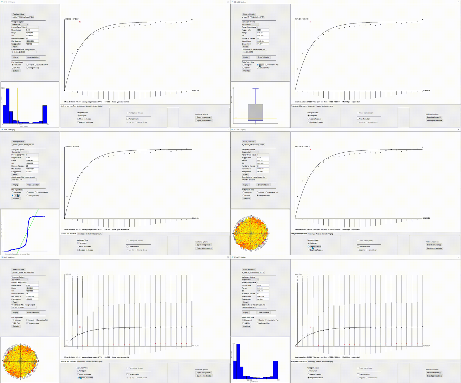
In the lower left area of our Kriging window you will see a small graph which, depending on the setting, shows a representation of the descriptive statistics.
Under histogram you see a bar chart over the classified value ranges with the class division of the values on the x-axis and the number of values in a class on the y-axis. It can also be generously called a "histogram" because the class division covers the same interval at every point - so the class width is the same everywhere. The number of values in a class correlates with the relative number and can be plotted on y. The class division is calculated in a simplified way according to scott. The yellow vertical line marks the arithmetic mean. If the input values only contain integers and these only cover a spectrum of less than 15 different numbers, the class width is set to 1 because we assume that this could represent classified data. This is a conservative approach and may not fit the character of all data.
Under [***Boxplot***](https://en.wikipedia.org/wiki/Box_plot) you can see the boxplot for the data. The yellow horizontal line marks the median value.
Under cumulative plot you see the range of values on the x-axis and the quantiles (0-1, normed cumulative frequency) of a value plotted on the y-axis. The plot shows the input values and does not calculate a curve fit.
Under QQ Plot the quantile-quantile plot is displayed. This is a simplified visual check of whether the distribution of your input values is close to a normal distribution. Since Kriging estimation is based on weighted mean values (explanation below), you will get more plausible results if your data is approximately normally distributed. On the y-axis, the empirical quantiles are plotted against the theoretical quantiles of the standard normal distribution. The blue points correspond to the quantile pairs to the input values. The green line marks the ideal line if the empirical quantiles would match the theoretical quantiles exactly. The further the blue dots deviate from the green line, the less a distribution resembles the normal distribution. Note that the visual test cannot replace a statistical parametric test for normal distribution. In geology (unconsolidated sediments) we have to deal with data that is not normally distributed. It is possible for geologists to be satisfied with an approximation to a normal distribution and still carry out kriging. This decision is very dependent on the character of the input values, the accuracy requirement of the estimate, the geological structures and ultimately also the value density in the area as well as the area size. Note also that your input values may show artificially skewed distributions of the input values due to a clustered spatial distribution in the case of a well-structured geological subsurface to which the parameter to be estimated is bound, but the actual underlying parameter distribution would nevertheless be approximately normally distributed. Kriging can be a complex issue in practice and the application of estimation should be done with care.
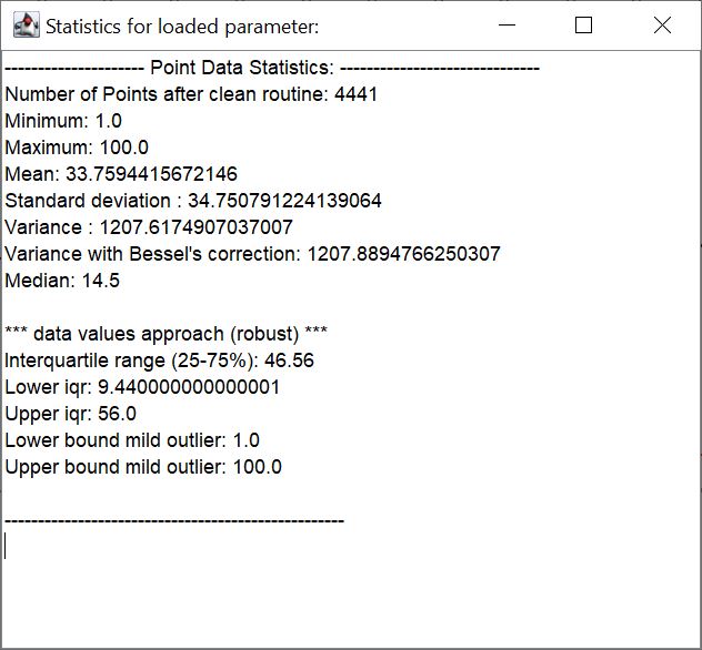
With the button statistics a small window opens, with which you can see the summary of the descriptive statistics in text form. You can export this text to your documentation with export point statistics or save it somewhere else with copy-paste.
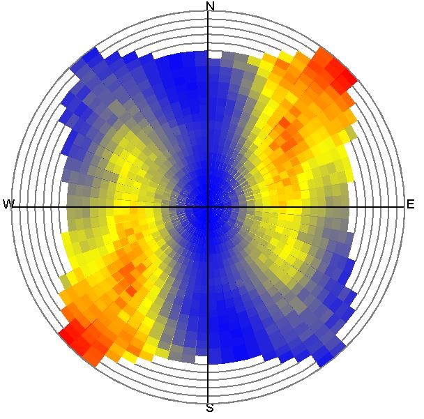
Under ***variogram map*** you can see the variogram map. Here the variances are entered directionally and for each distance class. The direction classes are created from north clockwise in 5° steps. Then the semi-variances are calculated per combined direction and distance class (see also [above](#experimentelles-variogramm)).
The distance classes with small distances start from the centre of the variogram map. Their boundaries are represented by a grey ring. The radius of the outer ring corresponds to the max. distance.
The colouring is relative to the interval of the minimum and maximum variances. Blue starts with the minimum variance value, yellow follows and finally red ends with the maximum variance value calculated in the classes.
With a variogram map you can visually detect directional anisotropies in your data set. In the figure a spatially structured distribution of parameter variance is shown. This is different in the example above. There, the variogram map shows rather a randomly fluctuating spatial distribution of the variance - i.e. no anisotropy.
The variogram map is created once as soon as you press the variogram map button for the current experimental variogram. With a large data set (several thousand points), the creation of the variogram map can take some time. It remains the same variogram map (so it does not cost any more time) as long as you do not calculate a new experimental variogram by changing the corresponding settings. In that case the variogram map must be recalculated.
¶ Transformations of the data
You can transform data if the distribution of your input values schould resemble more closely to a normal distribution. You will find functions for this at the bottom of the window in the tab analysis and transform.
.gif)
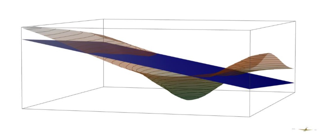
If you are working with 2D data, you can activate trend plane (linear). A linear regression is calculated over the input values before the variogram calculation (and also respectively the kriging). This produces a linear trend surface. The residuals, i.e. the deviations of the input values from the trend surface, are calculated. The residuals are used for all further calculations. In kriging, the final estimate is calculated back from the trend surface. This gives you an estimate that is not distorted by a global trend (external drift).
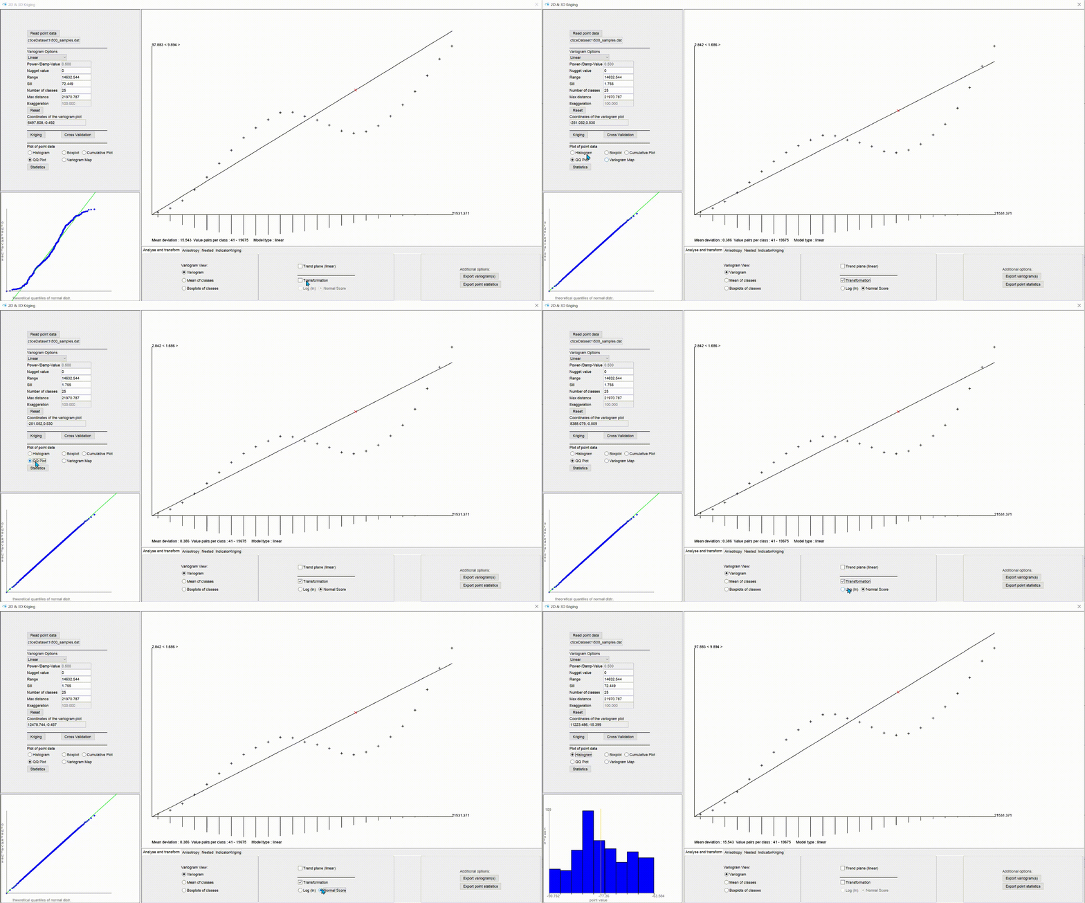
We offer further data transformations as log (ln) and normal score transformation. To do this, tick the transformation box and select the appropriate method. If your data set contains values less than or equal to 0, you cannot perform the log (ln) transformation. You will receive an error message. The normal score transformation makes use of the quantiles of the empirical values and those of the standardised normal distribution. According to the quantile of the input value, the equivalent value to the quantile from the standardised normal distribution is taken and used for all further calculations. As a rule, this transformation is quite robust. With some data sets, discrepancies can arise at the outer edges of the distribution. In this case, a decision to use or not use must be made. You should not perform a normal score transformation on small data sets. The back transformation of the final estimated values into the distribution of your input values uses exclusively linear methods.
With 2D data you can make a combination of trend plane (linear) and transformation. Within the SubSurface Viewer the combination always takes place internally in the correct order.
Note:
When kriging with the SubsurfaceViewer, the estimated values are brought back into the distribution of the input values with methods of back transformation. However, we have only implemented this for the estimated values themselves, but not for the kriging variance or standard deviation. Unfortunately, you cannot use these for your evaluation if you use a transformation.
To document the transformation, you can use the function export point statistics. A text protocol of the descriptive statistics of your input values and below your transformed values will be output.
¶ Fit theoretical variogram model
*The theoretical variogram model is the most important part of the kriging estimation. In order to decide and fit a theoretical variogram model, the experimental variogram is calculated in the first place. Read the section kriging below to understand exactly what significance the variogram model has for kriging estimation.
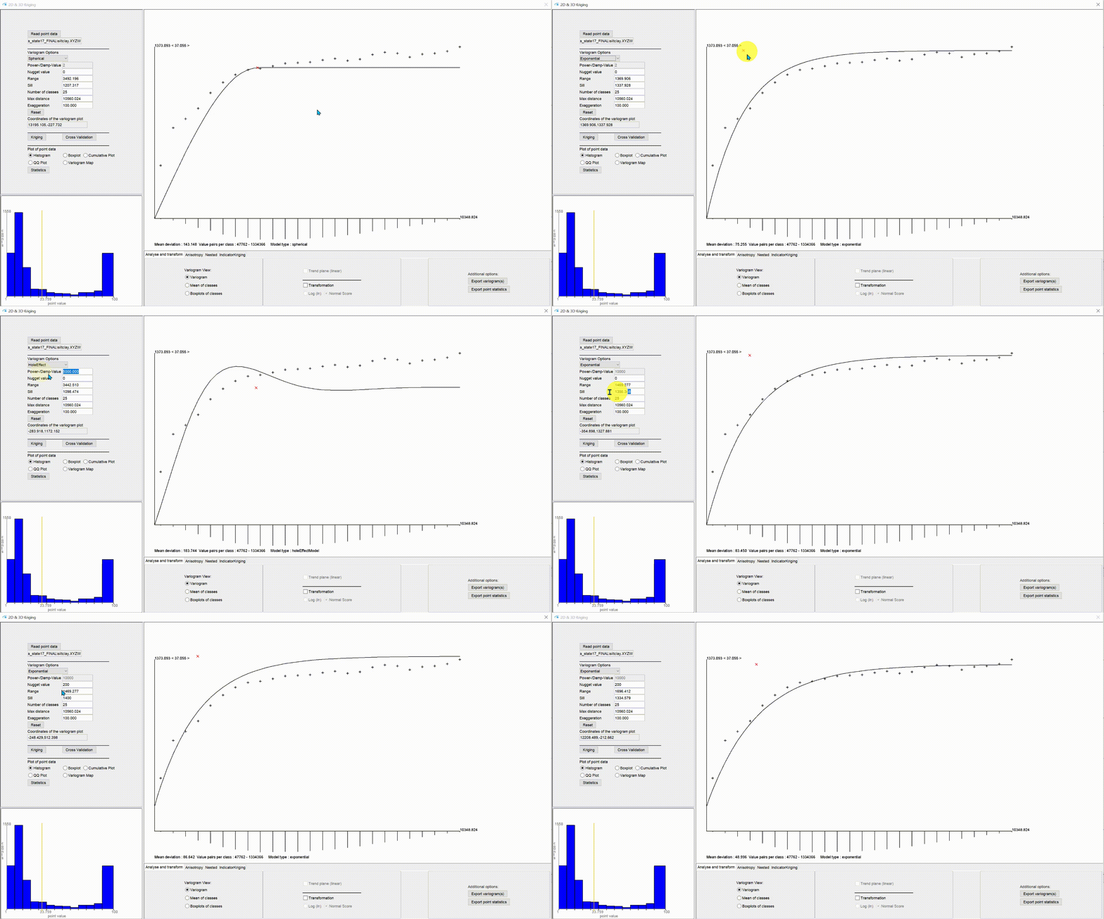
The central drawing field of the kriging window is interactive for the adjustment of the theoretical variogram model. You can click and hold the mouse and drag the theoretical variogram model into the correct position.
The corresponding values for sill and range will be updated automatically. The small red cross in the drawing field shows the position of sill and range in the graph. The sill corresponds to the position on the y-axis at the red cross. For constrained models, such as the spherical model, this value is theoretically the largest variance of the input values to be expected in the area. The value range corresponds to the position on the x-axis at the red cross and is to be understood in metres. From here, the theoretical variance no longer changes for bound models, as there is no longer any autocorrelation. This is why the term correlation length is often used. From this distance onwards, the variance of the data is no longer dependent on the distance between the pairs of values. In unconstrained models, such as the linear or exponential variogram model, sill and range nevertheless flow into the calculation formulae of the models, so tthey represent an essential component.
You control the selection of the type of variogram model via the dropdown list in the upper section of the left-hand options bar. The following are available for selection:
- linear (unbound)
- spherical (bound)
- cubic (bound)
- gaussian (unbound)
- exponential (unbound)
- pentaspherical (bound)
- spherical-exponential (special)
- hole-effect (special)
- power (unbound)
Refer to relevant literature for more details and recommendations on the variogram models. If you have a small data set, you can intuitively fit different variogram models and test them with cross-validations and result checks which model leads to the most favourable spatial distribution of your parameter.
The value entered under nugget value is another important input value for the variogram model. The nugget value determines the in-situ variance, i.e. the natural variance that is present in situ. This can include measurement error. In many cases it is 0. For kriging estimation, this means that exactly at the location of the input value, the input value is also estimated again. One speaks of expectation fidelity. If a value is set for the nugget, on the one hand the variogram model is shifted upwards at distance 0 on the y-axis, i.e. variance != 0 = nugget. On the other hand nearby input values have an influence on the estimated value at exactly the place of the actual input value. For more information read the chapter kriging.
The parameters sill, range and nugget affect the calculation formulae of the variogram models. The hole-effect model and the power model are the only ones with an additional calculation parameter. If you select one of these models, the upper input field power-/damp-value becomes active. If you have selected the hole-effect model, the value corresponds to the distance (in metres) from which the fluctuation of the hole-effect is damped. If the power model is selected, the value corresponds to the power factor of the model. For all other models the field is inactive.
The field coordinates of the variogram plot shows the variogram coordinates when you move the mouse in the central graphic field and supports you in the adjustment.
If you want to enter the corresponding model values manually, you can enter the numbers in the corresponding text fields. As soon as you have confirmed your entry with ENTER, the model is displayed updated.
At the bottom of the image of the variogram you can see the value mean deviation, which changes as soon as you change the variogram model. It corresponds to the mean deviation of your model from the semi-variances of your experimental variogram. It is advantageous to try to minimise this value. A true quality check of your fit should ultimately be completed with a cross-validation.
To document a variogram model adjustment, we have included the export of a simple text protocol. You can find the function under export variogram(s).
For the special cases of a variogram model definition in the anisotropic case and when using nested-variograms, read the corresponding linked sections.
¶ Anisotropy
You have the option of performing variography with anisotropy. Go to the anisotropy tab in the lower options area of our kriging window and activate the checkmark for directional. The radio buttons in the tab become active and two experimental variograms are calculated - one for all pairs of values that fulfil the search condition in the anisotropy direction and one perpendicular to the anisotropy direction or outside the search condition.
The search condition consists of the direction angle of the anisotropy direction of variogram in degrees from north (=0°) clockwise (as well as 180° mirrored to it), the opening angle of the search, which you can set with angle tolerance, and the bandwidth bandwidth. Move the corresponding sliders or enter a number in the corresponding text field. As soon as you have confirmed a field to the right of a slider with ENTER, it updates to the correct position. Here you have to press the "slide button" for a variogram recalculation. With bandwidth you set the maximum opening of the search condition. The variogram calculation is updated with ENTER.
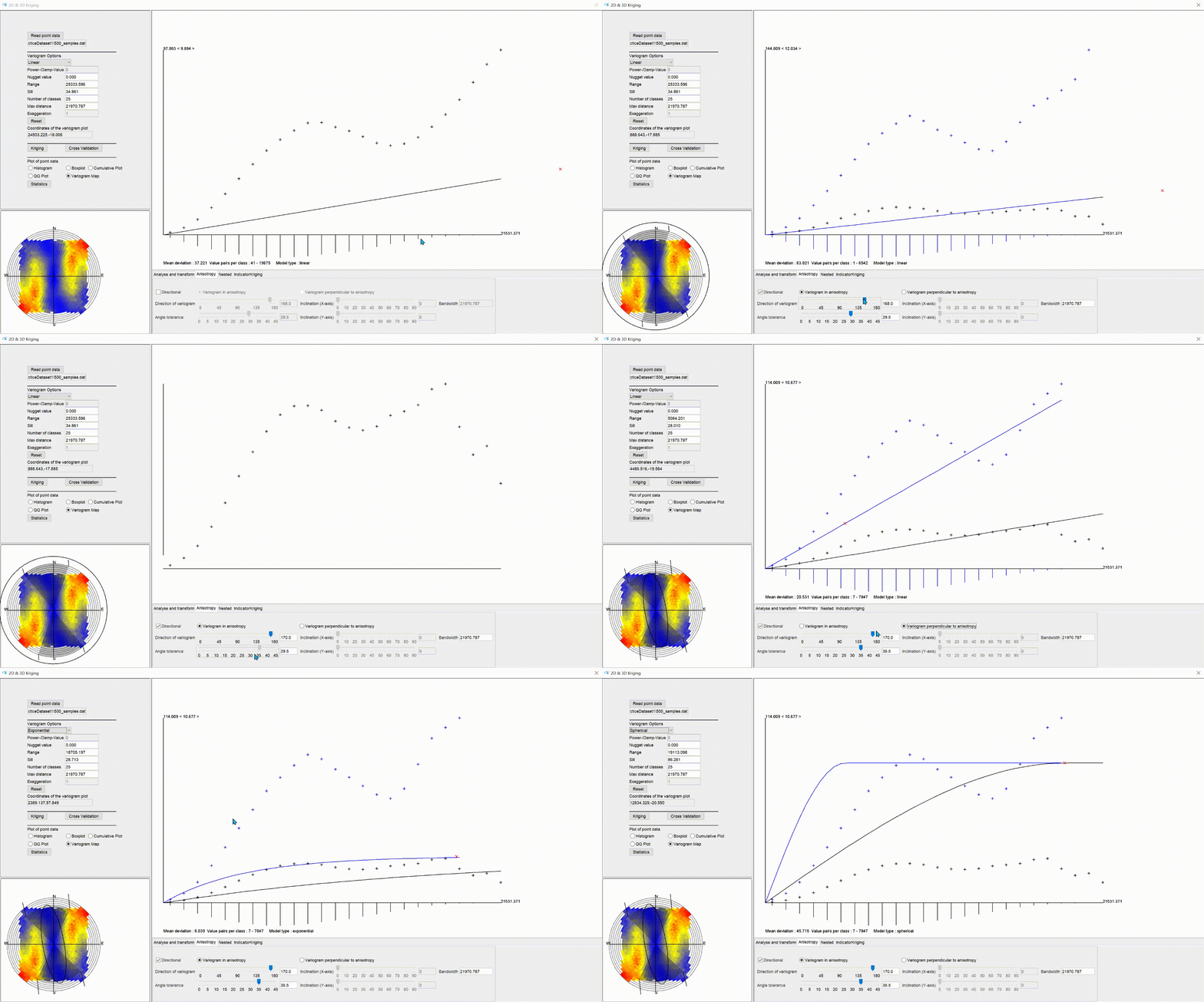
The experimental variogram in the anisotropy direction is shown in black and the one perpendicular to it in blue.
If you use the options in the tab analysis and transform -> variogram view, you will get two graphs. If you switch to mean of classes, the values in the anisotropy direction are darker red. If you switch to boxplots of classes, the boxplots in the anisotropy direction are grey and the others are turquoise.
It is recommended to switch the variogram map on the left to make it easier to find the anisotropy axis in your area on the one hand and to optimise the variogram adjustment by means of the variogram map on the other hand. Both are synchronised in the display in case of active directional options. You will see an ellipse (black) and the range of the opening angle as grey shading above the variogram map. Both will rotate with your direction of variogram setting.
The shape of the ellipse depends on the two variogram models that you set respectively. If you have selected a variogram model, one is shown in blue and one in black. You can adjust either on the variogram in or perpendicular to the anisotropy direction. To do this, switch back and forth between variogram in anisotropy or variogram perpendicular to anisotropy.
The two variogram models differ only in the correlation length range. The sill is the same in both, because the black variogram changes when you change the sill in the blue and vice versa.
The ellipse in the variogram map will change when you change the range values of the models. It shows the correlation lengths in and perpendicular to the anisotropy axis with its two ellipse axes. The final ellipse created by the different correlation lengths is crucial for the anisotropic kriging estimate. The opening angle and the bandwidth only help you to create and interpret the experimental variogram.
If you go in with 3D data, you have the option of setting the inclination for the X- and Y-axis, i.e. the angles of incidence. Use the controls inclination (X-axis) and inclination (Y-axis). These are inactive if you have loaded 2D data.
Note on inclination: We have introduced this function for the sake of completeness, but have not created a variogram map synchronisation for it. We concentrate on the lock sediment area and here the use of inclination is rather rarely necessary. Feel free to contact us if you think that a representation would be indispensable for your work. Perhaps we can consider this in future development.
When you have finalised your anisotropic variogram models, you can use the export variogram(s) function for documentation. Both models are documented in a text format.
¶ Nested variograms
In the lower options field of the kriging window is the tab nested, to create nested variograms. They are a linear combination of different variogram models. The individual variogram models are displayed in different colours. The final variogram model resulting from the linear combination is drawn in black. This is the decisive model for the kriging estimation.
.gif)
As soon as you have activated the check mark nested variograms, two variogram models of the previously set type are created. In the field number of nested structures you see a 2. With the button add nested structure you add further variogram models. The number of structures is unlimited. You enable the editing of the individual models via the dropdown list on the right under work with nested nr. If you change the variogram type in the dropdown list for variogram types in the top left-hand corner, the variogram type changes and the resulting variogram model changes immediately.
The active variogram model is always drawn a little thicker than the others so you can find it in the interactive window. With the button delete active nested structure you can delete the currently active variogram model.
If you do not have the additive calculation function active, relative weights can be assigned to the different models. To do this, move the slider choose weight of variogram back and forth. Since the weights are normalised as a whole, you may have to adjust the weights of all variogram models a to get a good result.
With the additive calculation the weights are irrelevant. Each variogram model has the same weight. The models are added linearly. You can see this immediately in the position of the black result model when you activate the function.
When you have finalised the nesting variogram, you can use the function export variogram(s) for documentation. All the models used, if necessary with their weights, are documented in a text format.
¶ Cross validation
When you have finished your variogram model definition, we recommend to calculate a cross validation before the actual kriging estimation. You can do this by clicking the cross validation button on the left-hand side. A simple window will open.
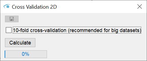
Here you can check 10-fold cross-validation if your loaded data set contains many thousands of points. If the check mark is not set, a leave-one-out cross-validation is calculated. It means that one point is always removed from the dataset, the kriging-matrix is built up with the remaining points, and a value is estimated exactly at the position of the omitted point. This is done for all points in the input dataset. Subsequently, the deviations of the real data value compared to the estimate are calculated and summarised in a table. A window for saving this table will open automatically when the calculation is complete.
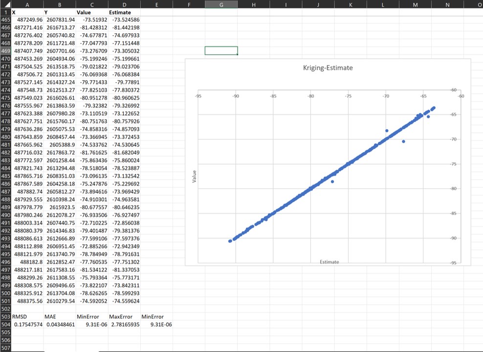
The table contains information on the root mean square deviation (RMSD = root mean square deviation), the absolute mean error (MAE) and the minimum and maximum error calculated. If you open this table with Excel, you can create a graph that shows the values of the input data on the X-axis and the estimated value on the Y-axis (or vice versa). If the points entered scatter more or less around a straight line, the theoretical optimum (estimated value = original value, deviation = 0), your kriging estimate might be acceptable. You should investigate whether you agree with the amount of deviation.
The respective XY coordinates of the points are attached to the table. You can load this table into the parameter manager to get a spatial view of your deviations, for example.
If you do a 10-fold cross-validation, then the same procedure is followed as already described above, except that instead of always removing one value, 10% of the record is removed. These are randomly selected, ensuring that each point is part of the 10% record removed once.
Note: We have kept the cross-validation tool simple as this has not been required otherwise in our previous projects. You cannot cross-validate for the case of reducing the next points used (see explanation here) to build the kriging matrix. All input values are always used for the cross-validation. The standard deviation of the estimators is not exported. If you think we should retrofit this in our future developments, feel free to contact us.
¶ Kriging
Now you can do the actual estimation after your completed variography and cross-validation. Use the kriging button on the left side of the kriging window.
If you have loaded 2D data, the output will be a grid. If you have loaded 3D data, the output will be a regular voxel model. You can read about the available output formats here: for raster and for voxel models.
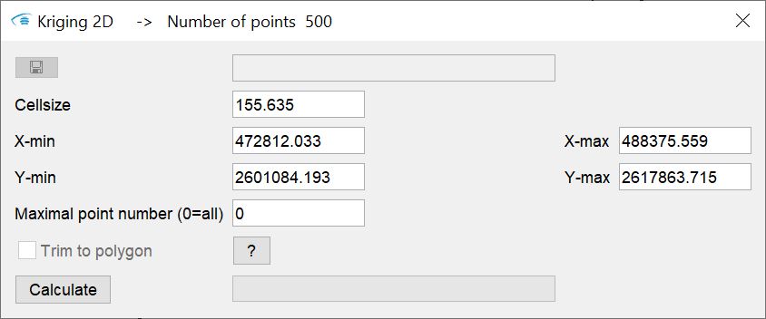
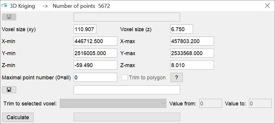
You can specify the dimension of the output raster or the output voxel model in the window. If you have stored a polygon, e.g. an area boundary in the buffer, the field trim to polyon becomes active for selection. If you check the box, the estimation will only take place on raster cells or voxels that are within the polygon.
With 3D kriging you still have the option of loading a master as an output voxel. Load an existing regular voxel model. This determines the geometry of the output. The kriging results are added to the existing voxel parameters. If you want to estimate on certain voxels, you can use the trim to selected voxel field. Use the dropdown list to select the parameter from the master voxel model on which you want to filter. Enter a value interval on the right. An estimation is performed where the voxels of the master model have values for the selected parameter in the specified value interval. You can use this function for an intra-layer kriging. This is explained in this article.
Press calculate to start the estimation.
The process of Ordinary-Kriging will be explained briefly:
- The kriging matrix is generated. The distances of all points or the maximum number of points (maximum point number (0=all), see below) are calculated. Based on these distances, the associated variance is calculated from the variogram model. This is important because you no longer have the experimental variance here, but the variance of the variogram model.
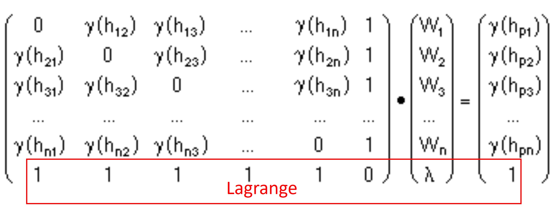
Internalise the ordinary kriging formula in matrix notation. y(hi) corresponds to the variance from the variogram model for the distance value of the value pair, or the distance of the value to the estimation point (see 2.).
Your choice and fitting of the variogram model has a high relevance for the entire estimation. On the diagonal (from top left to bottom right) is the variance of the input value with itself. Here you find the value of the nugget effects. If this is 0, there is also a 0 everywhere in the diagonal. - The distance of all input values to be used to the estimation point is calculated. According to the distances, variances from the variogram model are calculated again and written into a vector. You can see it in the illustration of the formula on the right-hand side after the equal sign.
- In the equation set up in 1., is still a vector that has not yet been explained. This is the vector of weights to be solved during the kriging process.
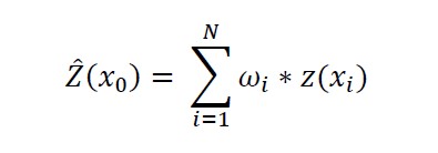
The weights are used to calculate the weighted mean of the input data used and the variance at the estimation point. The weighted mean is the actual estimated value. The variance calculated at the same time is the kriging variance from which the kriging standard deviation is derived.
In summary, kriging is the solution of a linear system of equations.
To ensure that the weights sum to 1, the outer last members of the matrix are filled with 1. In the vector for the variogram variances at the estimation point, the last row is filled with 1. This enables the solution of the so-called lagrange parameter, which is located in the last row of the weight vector. It is also used as a correction factor in the calculation of the weighted mean. To solve the system of equations, the kriging matrix must be inverted. Search online for the keywords "inverse matrix" and "Gaussian elimination algorithm" for help. Depending on how many points you have to use to build the kriging matrix, this process takes some time.
Finally, the estimated values with their standard deviation (or variance) are written into a given grid or voxel model and are ready for your analysis.
Note that the construction of a kriging matrix can take longer if there are a lot of input values. If it takes too long or the matrix would be too large for the memory of your computer, you should reduce the number of input values used to build the kriging matrix. The corresponding field can be found under maximum point number (0=all). If you set a 0 here, all input values are used. If a number is set here, the input values are sorted in ascending order based on their distance from the estimation point. Only the closest points, according to the specification of the maximum points, flow into the kriging matrix. Check your results carefully, especially if you have a well-structured background to which the parameter to be estimated is bound and at the same time a rather clustered spatial distribution of your input data.
Note: When reducing the points used to build the kriging matrix, note that a separate matrix must be built and also inverted** for **each estimation point. If you use all input points, the (large) kriging matrix is built once, inverted and used again for each estimation point. Thus, under certain circumstances, an unfavourable choice of the maximum number of points can lead to higher calculation times than with the choice of all points.
Once the calculation is complete, a window will open to save the result. In 2D kriging, two raster files are generated. One contains the estimate itself, the raster marked .sdt. contains the associated kriging standard deviation.
If you have performed 3D kriging, you will get three new columns in your newly created or extended voxel model. You define the name of the estimation parameter via a simple input dialogue that appears when you finish the calculation and define the file. The estimate and the associated kriging variance and kriging standard deviation are written to the voxel model with this parameter name.
Important note: You should view the info-window after completing the kriging estimation. This is where we log the kriging process. Hints are given about unusual weights (sum of weights not equal to 1) or unusual lagrange parameter values. So this gives you hints on how to rank the goodness of your estimate.
¶ Indicator Kriging
In the lower options field of our Kriging window you will find the tab indicator kriging. Indicator kriging can be used if you..:
- ... are dealing with skewed or multimodally distributed parameters,
- ... want to perform an estimation for a categorical data set,
- ... want to estimate the probability of exceeding or falling below a limit value.
In short, categorical indicator kriging is estimating the probability of occurrence of a particular class, indicator or category. It is the estimation of the relative probability of occurrence of values in a certain value interval. For example, the values within the interquartile range have a relative probability of occurrence of 0.5, which means that these values occur in 50% of the measured samples. If we measure again and the distribution remains the same, then we have a 50% chance of measuring values within the interquartile range. The special feature of indicator kriging is the consideration of occurrence probabilities with spatial correlation considered. Categorical indicator kriging can also be performed on the index values of an already predefined category, such as the layer ID of a specific geological unit from the GVS-file. You get the relative spatial probability of occurrence of the particular index at the estimation location.
Another possibility is to use indicator kriging as a limit value observation. You estimate the relative probability of falling below or exceeding a value at a certain location. It is the estimation of the relative cumulative probability of occurrence of a limit value. For example, if you take the value at the upper interquartile limit, i.e. quartile 75, then the cumulative probability of measuring values below or equal to quartile 75 in a new measurement is 0.75. You have a 75% chance of this condition being achieved.
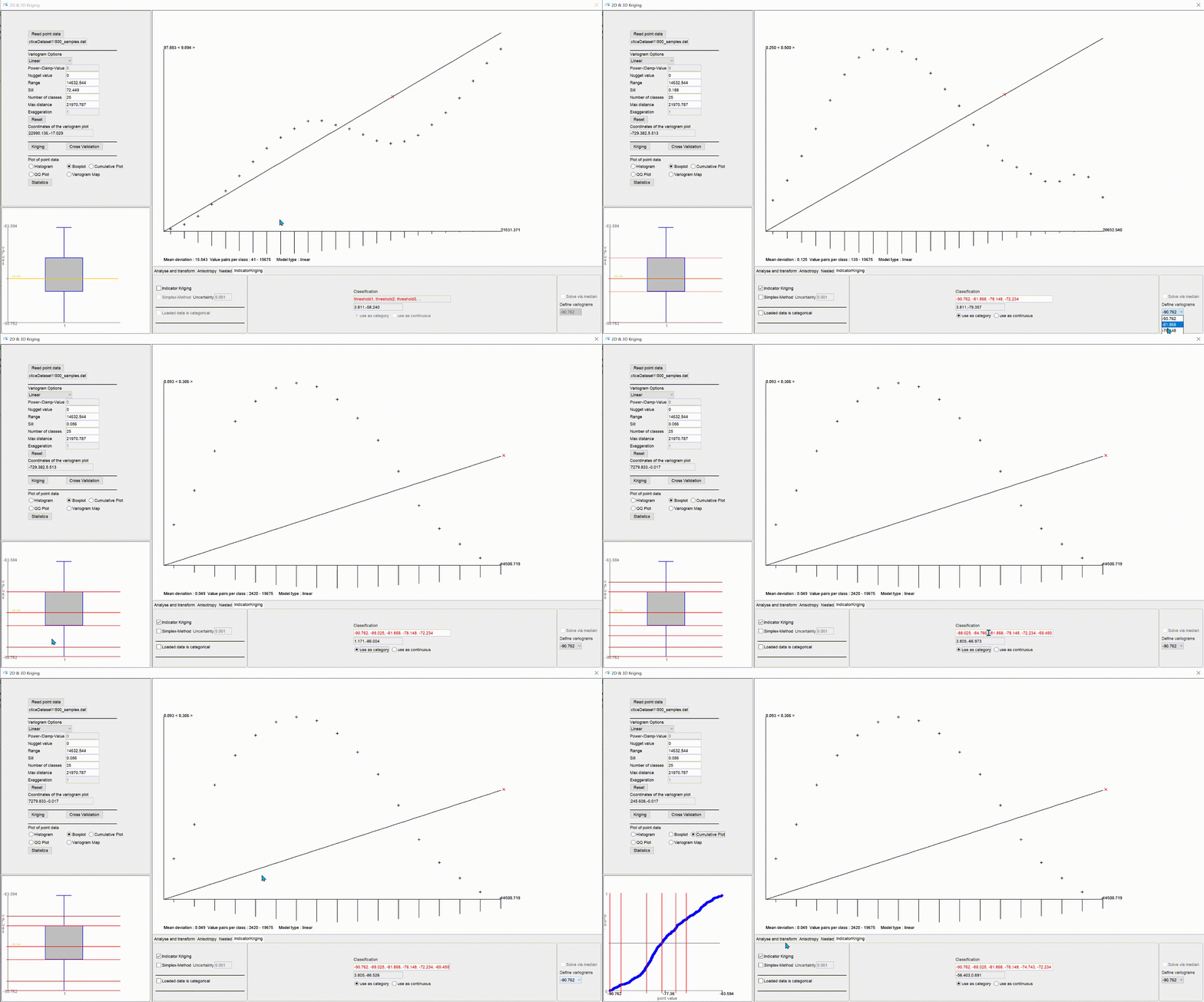
Use the button in the lower middle options field use as category to activate the categorical indicator rigging. With the button use as continuous you set the limit indicator rigging active. With the check mark at loaded data is categorical you tell the system that you have already loaded categorical index values as input data set.
As you may have guessed from the previous explanation, you can load both continuous and categorical data for indicator kriging in SubsurfaceViewer.
If you want to go in with a continuous data set, you can classify this data internally, or divide it into limits. To do this, set the checkmark for indicator kriging to active. A classification is suggested on the basis of the robust descriptive statistics. You can see this when you look at the statistics window for the histogram, the boxplot or the cumulative plot on the left. You will see red lines marking the lower limits of the classes or the limit values. The best way to understand the proposal is to make the boxplot visible, because the proposed class division uses the median, the quartiles 25 and 75 as well as the minimum with active use as category or the maximum with active use as continuous. The initial proposal divides the data set into equal parts for the time being.
For use as category, divide the record with the lower limit of the class/category. With use as continuous you share with the upper limit. For loaded data is categorical, each individual index record forms its own class.
You will see the class limits listed in the middle section of the lower options bar in the classification text box.
Note: Since you need to define a separate variogram for each class or limit case, the same values are listed in the dropdown list under define variograms on the right-hand side. Switch from one experimental indicator variogram to the next with this list.
If you want to define classes or limits, enter the corresponding lower/upper limits in the text field classification. Keep the format of the proposal - the values must be entered comma-separated. As soon as you confirm with ENTER, the dropdown list for switching the corresponding variograms as well as the red lines in the statistics plot are updated. You can define classes interactively in the statistics plot. To do this, double-click on the corresponding position in the plot and a boundary will be added, which you will see both in the text field and in the dropdown list. Right-click on a red line in the statistics plot to delete the class boundary. For orientation, you will see the coordinates in the statistics plot below the classification text field when you move the mouse there.
Note: If you have made a change and want to return to the classification proposal, uncheck indicator kriging and activate it again. This will take you back to the default setting.
Note: The list of (class) limits is always sorted from left to right after confirmation.


Here you can see the formulas for the indicator transformation that takes place internally as soon as you have confirmed a classification or limit definition.
The indicator transformation of the data in categorical indicator kriging has the effect that in the case of fulfilment of the class condition (values lie within the class interval or corresponding exactly to the index of the category), a 1 is set at the locations of the input data and a 0 in all other cases. If we are dealing with a limit value consideration, 1s are set everywhere where the values are less than or equal to the limit value, and 0s everywhere else. This is done for each class or limit value.
With 4 classes/limit values, you have 4 new data sets in the memory. From these, 4 independent experimental variograms are calculated for which you have to define 4 variogram models. Switch between the variograms to the internally transformed data sets via the dropdown list under define variograms. Variogram analysis and creation remains as known and described above.
Note: Note that a boxplot representation of the variances for the distance classes is obsolete, as the individual variances between the pairs of values can only be 1 or 0. Thus boxplots cannot be represented.
In the case of the limit value observation, you have the option of setting a check mark at solve via median. It will be shown only one experimental variogram for which you have to define the model, namely for the median limit value. If your spatial variance of the occurrence probabilities for your set limits is similar to that of the median, i.e. the experimental variograms are very similar, you can calculate the kriging estimate with the variogram model associated with the median. This may save a lot of calculation time because the kriging matrix is only built using the data set and model associated with the median and then reused for each indicator. This method is called median indicator kriging.
Note: If you have the maximum value of all input values in the dropdown list active in the limit definition and your experimental variogram shows nothing, do not be surprised. For the maximum value as the limit value, the limit value condition is fulfilled at all locations, since all values are less than or equal to the maximum. So a 1 was set everywhere and thus there is no variance at all. We have added the maximum value to our proposal because it can be used to complete the theoretically derivable cumulative probability curve at the estimation location. No kriging is calculated for the maximum limit value, but each raster or voxel cell contains a relative probability of 1 in the result for this maximum limit value. This brings advantages later in the evaluation of limit value observations as well as the long-term traceability of the estimate.
If you activate kriging as usual, for each indicator (class or limit value) a run with ordinary kriging is carried out on the corresponding transformed data set. In the window for starting the calculation, you still have the checkmark multi-threading for selection. The calculations are carried out in parallel on a maximum of 4 different threads. Everything else will be as you can read in the section kriging.
In the output, you will get a grid or a column in the voxel model for each class or limit with the estimated relative probability of occurrence with values between 0 and 1. The names for the columns or grid files are composed by the parameter name you entered and the respective (class) limits you set during variography. If you have performed categorical indicator kriging, you will find an additional column or grid with the addition _mostProbable. At each estimation location, the class with the highest probability of occurrence is written into the grid cell or voxel with its class ID.
Important note: You should look at the info-window after completing the kriging estimation. This is where the kriging process is logged. Hints are given about unusual weights (sum of weights not equal to 1) or unusual lagrange parameter values. This will give you hints how to rank the goodness of your estimate.
The setting simplex method will be explained here. It ensures that the estimated probabilities of occurrence of the individual indicator kriging runs are consistent in the result and that a plausible cumulative probability function could be theoretically derived at each estimation site. The method was taken from Tolosana-Delgado, Pawlowsky-Glahn & Egozcue, 2008: "Indicator Kriging without Order Relation Violations.", Math Geosci(2008) 40:327-247. The value Uncertainty is also explained there. Note that the implementation of this method was experimental and has not yet been fully tested.
If you do not check simplex method the method described by the function ordrel.for from the GSLIB library, which is now openly accessible, is carried out with slight adjustments. The correction, like the weights and the lagrange parameter, is logged in the info-window.