To learn how to create profile sections, follow these links:
- Synthetic Sections,
- Toolbars and there 2D-View and 2D-Cross-section View,
- Construct Profile Sections,
To get to the descriptions of the general settings of profile sections, follow this link. Here you will find many properties of the profile sections that are useful for your modelling.
The profile sections have the general options that all SubsurfaceViewer objects have. You can find out more about this here.
In this article we will deal exclusively with the functions you can reach via the right-click context menu and the options you have in the window.
**Unlike all other SubsurfaceViewer objects, you get access to the complete context menu in the object tree of the cross-section view. With other objects you were used to going via the tree in the 2D view.
Note: Since our regional models sometimes have very long sections, the complete drawing of a section can be time-consuming. Therefore, in large areas you will see lines at first. Press the Refresh button of the Toolbar or use the context menu to update sections. This applies to drawing modified lines as well as the fill polygons linked to them. So you need to use the refresh options more often.
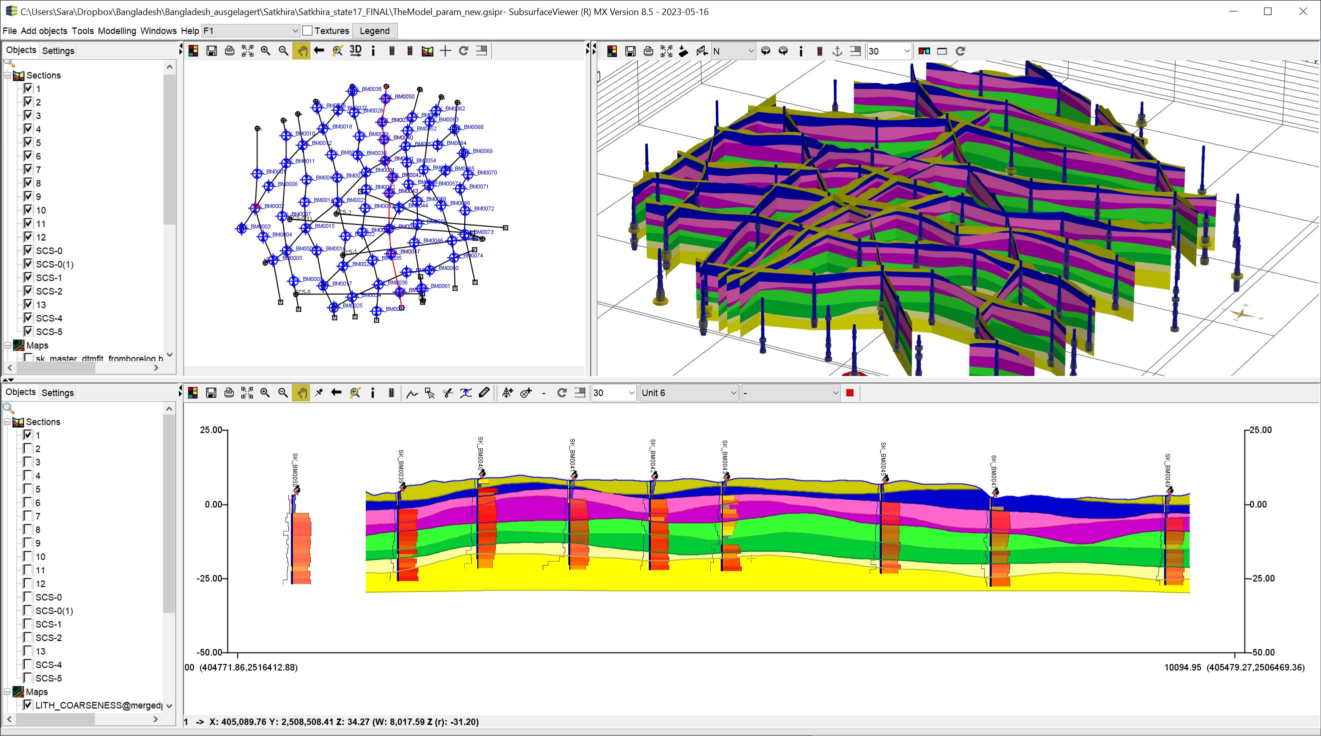
¶ Options in the profile section window
With a right click in the profile section window you have the option to place a note at any coordinate. Such a  symbol then appears. If you right-click on this symbol, you can subsequently edit or delete the corresponding note. With
  Move notice in the toolbar you move the note.
If you right-click on a constructed line, you have a menu of line options available. You can find these options in the general settings for all lines. Have a look at the article on the context menu below.
A right click on a hole or coordinate that you used to construct the profile section opens a small menu that allows you to delete the break point. This can change your constructed lines.
You can move the profile with active  button and click+hold.
¶ The context menu
Open the context menu for individual profile sections with a right click on the name in the object tree of the cross-section view.
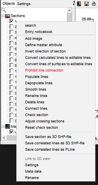
Various profile cut options are available: cut orientation for loading a background image or grid, conversion options for lines, line editing tools for the entire cut and export functions.
Use Settings to customise the settings of this section.
Follow the sub-chapters to learn more about the functionalities.
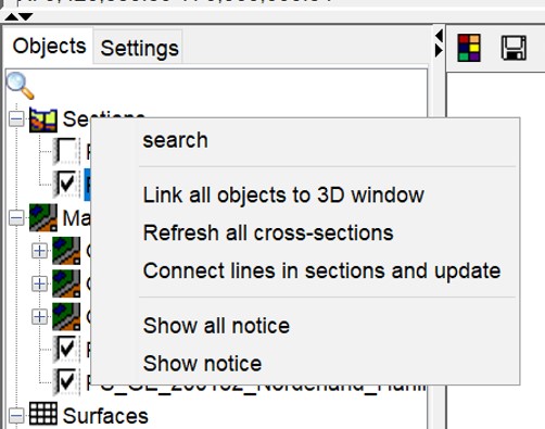
If you right-click on the  icon further up the tree, a menu opens that offers functions for all profile sections.
With Link all objects to 3D window you send all profile sections to the 3D view.
With Refresh all cross-sections you update all profile section drawings. Keep in mind that this may take some time for large areas with long sections and dense profile section meshes.
Connect lines in sections and update is a function to connect line segments with the same naming. A distance of 1 metre is set as a condition. The sections are updated. Note that you can suppress the line connection for individual profiles.
With Show all notice you can view all notes that were saved in the sections as a summary in Excel. The Excel window opens automatically for this.
With Show notice you can see the general notes on profile cuts. If you want to know more about Notes, follow the link.
Note:
If you want to add notes to the section, right-click anywhere in the profile. There you have the option to choose between Show all notices (to the profile) and Add notice. With the latter option, you add a note that immediately appears in the window with such this
symbol. If you click on this symbol, you can change (Edit notice) or delete (Delete notice) this note in the context menu that opens. With the corresponding symbol in the Toolbar, you can move this notice to an understandable place. Conceptual modelling requires a lot of interpretation by the geologists. There may be uncertainties or changes that would not be directly comprehensible to others without documentation. With the notes, it is easier to work on models together with third parties, because you save your documentation directly with the model.
¶ Add image
Insert a background image in raster image format or directly an ASCII raster (*.asc, *.rst) into a section. The images/raster can be fitted into the cut by dragging, compressing and tugging as required. Use this to perform georeferencing of vertical sectional images.
Note: You can fit seismic section images here and enter the results of a seismic survey. Check how much memory usage you are allowed, with about Subsurface Viewer (R) MX under Windows. If you are able to convert your seismic sections to ASCII rasters, you will have some additional colourisation options available in SubsurfaceViewer.
If you have integrated an image, do not forget to check Background image in the Profile Section Settings or in the General Section Settings. You can delete an image using the right-click context menu with Delete image.
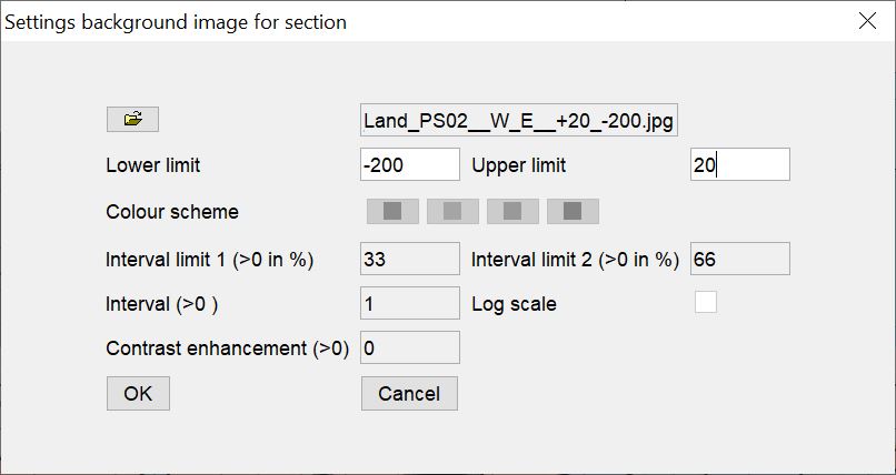
If you want to load an image or grid, the window shown opens first. With Lower limit and Upper limit you set the vertical extension that belongs to the marker. If you do not know this, because the section may also contain borders in the image, you can accept the suggestion for the time being and adjust the image accordingly later.
The options below are relevant if you load ASCII raster data. You can create a four-level colour palette with Colour scheme, set intervals for the value intervals for colouring, select a logarithmic scaling with Log scale and trigger a contrast enhancement (*Contrast enhancement (>0). These options can be useful, if you want to do your visual analysis of geophysical section data (e.g. also geoelectromangnetics) with this.
Press OK when you finished your settings.
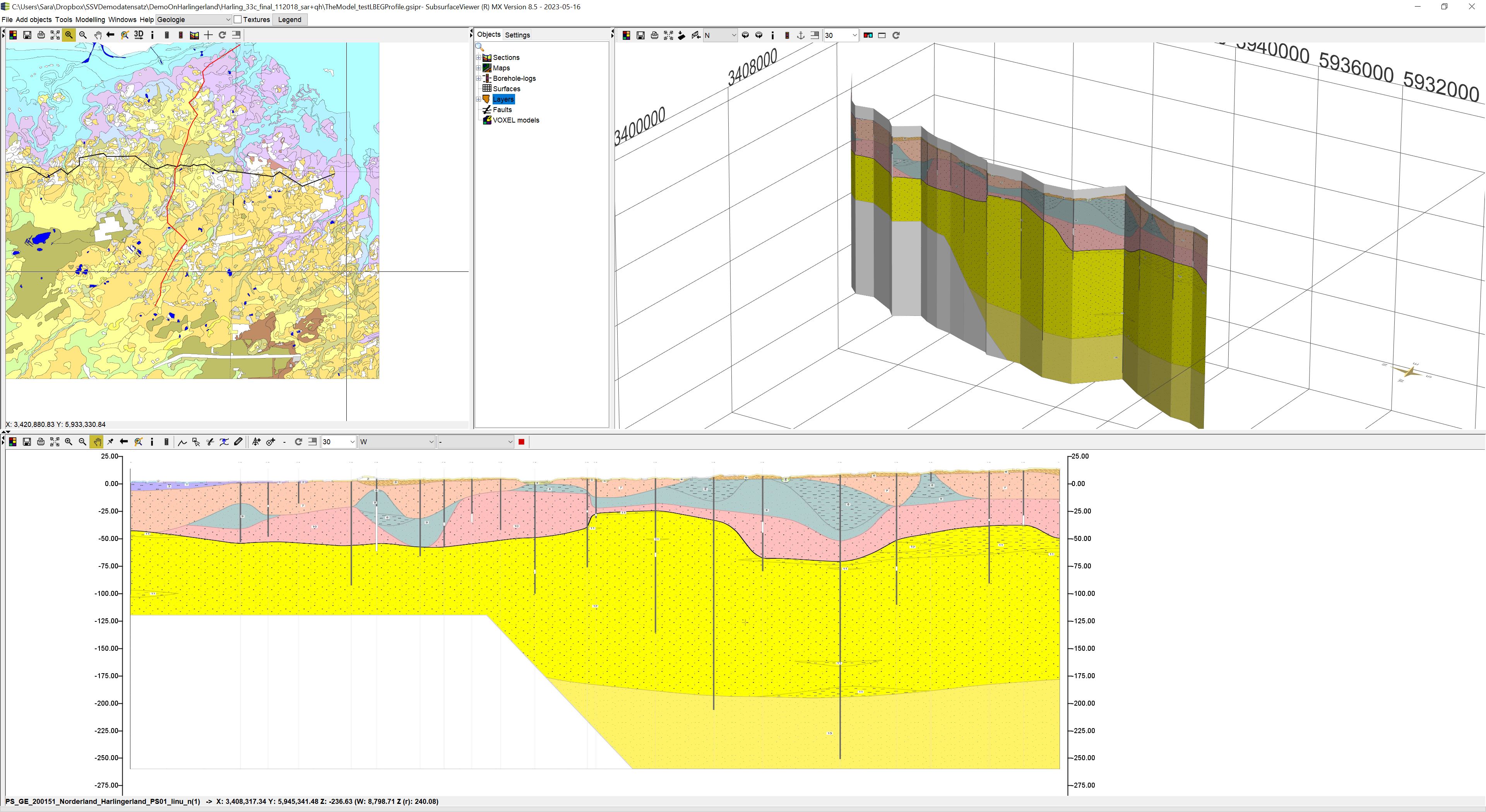
The result of loading an image as a JPG is shown here.
Note: The example was provided by the hydrogeological department of the Landesamt Bergbau, Energie und Geologie des Landes Niedersachsen (LBEG).
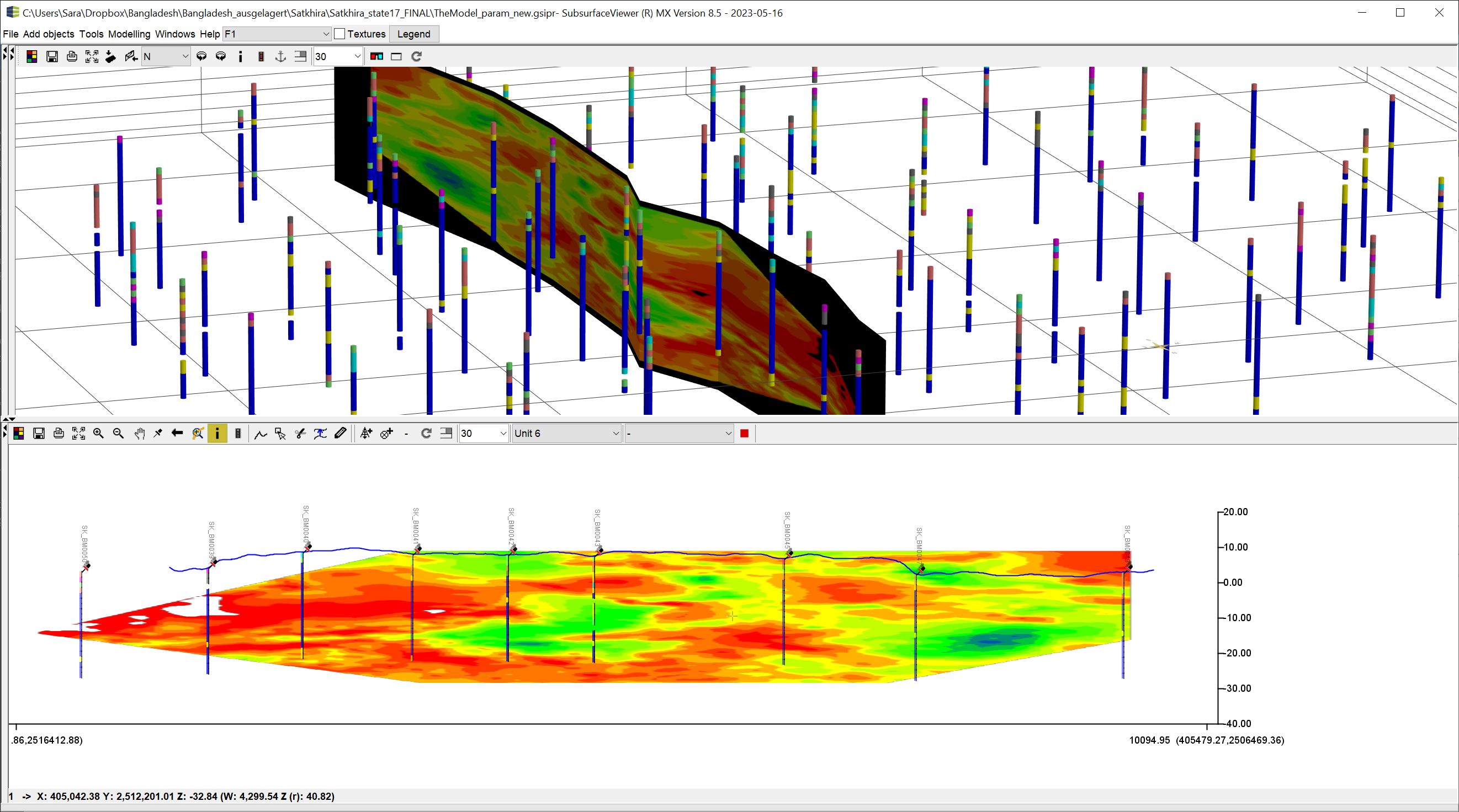
Here is an example of loading an ASCII raster with the colour palette set.
Note: The background raster in the example image is synthetic and not based on any real measurement.
If your image or grid is not yet in the right position, you can open Adjust image in the context menu.
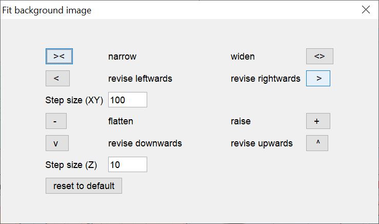
A dialogue opens with which you can make the adjustment. The position and extension, as well as the positioning of the image will update when a button is used.
With narrow you shorten or compress the image/raster horizontally.
With revise leftwards you move the image to the left.
With revise rightwards you move the image to the right.
With widen you stretch the image/raster horizontally.
With step size (XY) you specify in metres how much you want to shorten or stretch (horizontally).
With flatten you compress the image/raster vertically.
With raise you stretch the image/raster vertically.
With Step size (Z) you specify in metres by how much the image should be shortened or stretched (vertically).
With reset to default you return the image to its original configuration when loading.
¶ Define master attribute
This is a tool to define a profile as decisive. It is a master profile and needs more attention in modelling. In addition, this marking can help to distinguish master profiles from auxiliary sections. You can see whether a section has been marked as Master in the title of the dialogue that opens.
¶ Invert direction of section
Inverts the direction of the cut. Use it if you want to add a hole or coordinate to the beginning of the profile. Invert, then attach the hole/coordinate using the appropriate buttons in the Toolbar, and invert back again. You might have to invert a section if a background image is to be loaded which is oriented the other way round.
¶ Convert...
¶ Convert calculated lines to editable line
This converts all lines of the layer bottom edges of the already calculated or imported geological layers into editable lines. The lines need to be assigned with the correct names. This function is useful if you have imported external model data and want to edit them.
¶ Convert lines of surfaces to editable line
This converts all lines of all loaded surfaces (TINs and elevation raster) into editable lines. The lines do not get a correct name assignment. This needs to be done later. This function can help you to edit further external model data.
¶ Prohibit line connection
This function is important if you have 3D line shapes converted to profile sections. It can happen during the conversion that lines made to draw lenses get the same line names as the main layer bottom edges. This leads to errors in the automatic line linking based on line names and distance of the nodes. In the SubsurfaceViewer the lenses must receive their own entry and name in the GVS-file. Since automatic line linking is triggered when loading a model with profile sections, this must be suppressed before saving such profiles.
¶ Allow line connection
If the suppression is active, you will see Allow line connection in blue in the same place in the context menu. This enables the connection, which we recommend before you go into the final calculation of your layers.
¶ ...lines
¶ Populate lines
Increases the node density for all lines in the section to a target distance in metres.
¶ Depopulate lines
Thins out the node density for all lines in the section to a target distance in metres.
¶ Smooth lines
Increases the node density for all lines in the section to a target distance in metres, but uses a spline algorithm to make the line more curved.
¶ Rename lines
Assigns a new name to all lines in the section with a specific name. This can be useful, if you have changed the GVS-file or used Convert lines of surfaces to editable line.
¶ Delete lines
Deletes all lines with a specific name.
¶ Connect lines
Connects all lines in the section unless you have Prohibit line connection active.
¶ Check section
The function is described here. It is only valid for this section.
¶ Adjust crossing section
This function adjusts discrepancies that exist at profile crossing points (crossing points) in the intersecting profiles. Be careful with this function, especially if you have a very dense profile intersection network with many crossing points.
¶ Reset check section
Use this to reset Check section markers.
¶ Save as...
¶ Save section as 3D SHP-file
Saves the polygons of drawn geological layers into a 3D polygon shape.
¶ Save correlated lines as 3D SHP-file
Saves all editable lines with names in the section as a 3D line shape.
¶ Save correlation line as PLine
Saves all editable lines with names in the section as a GOCAD PLine-File.
¶ Settings
Note: When you open this window, you inform the system that this profile section will not have a general layout but an individual one.
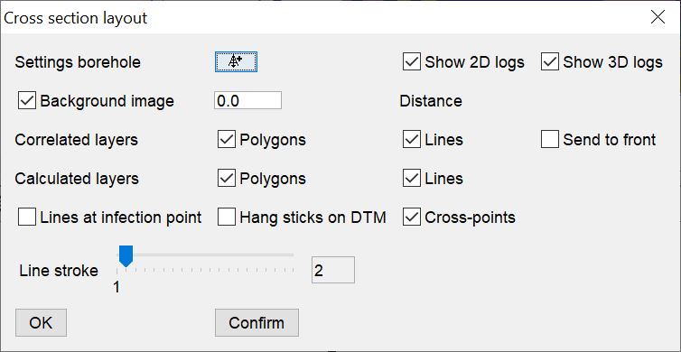
Here you have all the settings available that are described here.