In this chapter it is explained how to view or edit a model in the SubsurfaceViewer which is already created.
If you want to compare your models with the model contents of others, you face special challenges, especially if conceptual models have been created. We do not yet have the optimal solutions for this complex topic. However, we would be happy to discuss this topic with you. We are currently developing new solutions with modern methods (e.g. integration of AI methods). Contact us or send us an email if you are interested.
We have first compiled a few recipes, as briefly as possible, for migrating model data into SubsurfaceViewer.
¶ Import geological layers
- Create a GVS-file and a projectlegend for the external model data for the geological layers.
- Load a digital terrain model as TIN, e.g. like this.
- Create a Layer-Object for each geological unit.
- Load for each layer-object via context menu -> extra functions optionally the layer lower edges and, if you have, the layer upper edges from these formats.
- (optional) If you had no layer tops available, you can select calculate tops of all layer in the menu item tools. If you now notice implausible layer penetrations, you should consider using the advanced calculation functions for layers. Therefore, it is necessary that your layer model is completely based on triangulations.
Note, that you must load a DTM as a TIN if you have imported triangulations. If you have loaded rasters into the layers, the DTM can also be a raster. The raster dimension and resolution of each layer must match the loaded DTM raster in the project settings. If this is not the case, you need to create triangulations.
If you want to create editable profile sections from this model, follow these instructions:
- First construct the course of a profile section. If profile section courses were already integrated in the other model, you can load them as 2D-lines shape and convert them into profile section courses with create cross-section along 2D-lines. Use the context menu of the shape and read the linked article if necessary.
- Now use the functions Convert calculated lines to editable line or, convert lines of surfaces to editable line in the context menu of the individual profile sections. You can set and edit new nodes along profile sections.
If you want to create editable structure maps, follow this instruction:
- Create contour lines for the imported layer bottom edges at distances that get enough information about the surface structure.
- Copy these contour lines via the context menu of the corresponding surface object into the clipboard.
- Create a geometry2D object and enable it for editing.
- Paste the isolines from the clipboard into this object.
- Link the Geometry2D object to the layer to which these isolines belong.
- Now you can edit them.
- Edit from young to old and eventually use virtual erosion so that you get a consistent model.
Alternatively, you can extract the isolines of your layer in another programme and integrate them as line-shape. Here the copy-paste function works the same way. Read the upper section in the article structure map modelling.
¶ Import geophysical models
In this chapter it is described how you can work with geophysical models:
- Create and load voxel models with these formats.
- You can fit section images or ASCII rasters of your vertical measurements into profile sections.
- You can use the parameter manager if you have borehole measurements or other point data.
- You can load borehole measurements as LAS files.
- You can load surfaces as triangulations or height grids. With this you can either extract isolines as structure maps or convert the lines of the surfaces in the profile sections into editable lines. Look above in the section import geological layers. The procedures are described there.
¶ Load and match profile sections from third parties
- profile sections from other sources can be loaded as 3D line shapes of the layer bottom edges. To do this, follow the instructions in this article. It is best to try to assign the line attributes to the loaded GVS. You may have to rename lenses manually in the edit.
- Then fade in the constructed layer lines or other surface lines for adjustment.
- Use the buffer distance in the settings of the cross-section view to project nearby holes into the section.
- If necessary, load a polygonal image of your section as background image.
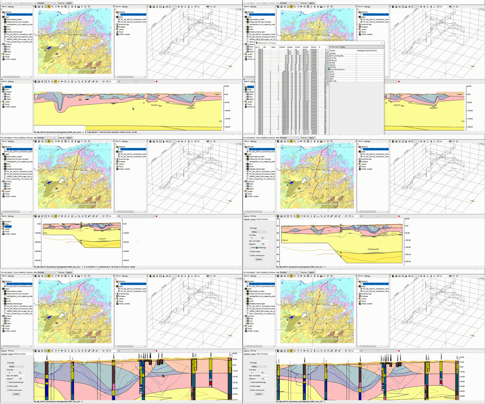
Below an example is shown.
The sections shown and the geological map were provided by the hydrogeological department of the Landesamt Bergbau, Energie und Geologie des Landes Niedersachsen (LBEG). The geological units in the section, which have been superimposed, are no longer valid, processing statuses of an area in Ostfriesland. These old statuses show that with conceptual modelling, there is always a great deal of room for interpretation, and things can change if, for example, new boreholes are added. This is especially the case with the 3D mapping of Quaternary unconsolidated sediments. If geophysical data are then added (dark blue line as lower edge of Lauenburg Clay), the real ones are probably somewehere in between. We would like to try to reduce uncertainties with our latest developments and to transport it to the users when passing models. Come and talk to us if you are interested in this topic.

¶ Convert 2D raster for depth horizons/layers into 3D voxel model.
Note: Using the same procedure as described here, you can also rewrite the calibration of a groundwater model into a voxel model. Therefor you need an import of geological layers and the calibration as a 2D raster for each layer horizon.
- Create a GVS file with the number of depth slices/layers and a name.
- Create a layer for each depth horizon.
- Take your digital terrain model as a raster and load it.
- Use the calculator for raster and subtract the values for the base depths of the depth slices from the DTM. In this way you create a stack of raster files that map the base of your depth horizons. These rasters always have the same dimension and resolution.
- you load the rasters created under 4. as layer bottom edges into the associated layers and save the DTM in the project settings.
- Calculate the top of the layers with tools -> calculate top of all layers.
- Export a regular voxel model with the function file -> export layers as voxel, which you load in immediately.
- Load all depth slices as geofactors into the project.
- Iterate the following procedures for each layer, which represent your depth slice intervals:
- Open the filter of the voxel model. Select a slice by ID so that the voxels belonging to the slice are displayed. Leave the window open.
- Open the calculator for Voxel Models. Leave the check mark calculation only on selected active. In the upper right corner, define a name for the parameter that you want to transfer from the raster data. Then select the appropriate geofactor from the list on the right with a double-click for the formula (see 8.) and confirm the calculation. Leave the window open. Please do NOT close the window or change the name of the output column now!
- Select the next layer as in the first point, then change to the second and so on.
- Save the voxel model in the calculator and you are done!
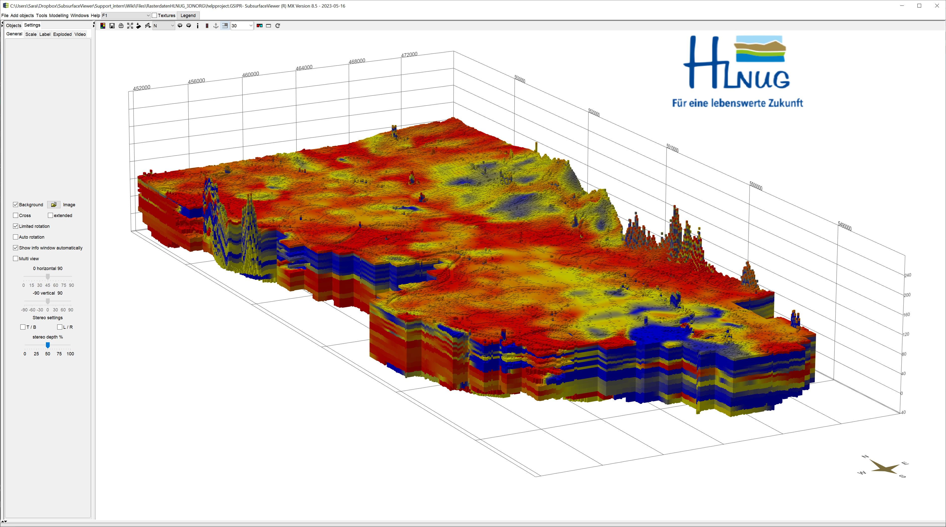
In the example, we have converted the depth slices from the 3D-NORG-project from the Hessian State Office for Nature, Environment and Geology (HLNUG) into a voxel model.
